High Performance Computing (Georgia Tech MSCS)
Lecture notes from my time in Georgia Tech’s MSCS program. Reference text: Introduction to Parallel Algorithms.
Contents
- Introduction
- Basic Model of Locality
- I/O Avoiding Algorithms
- Intro to Work-Span Model
- Comparison Based Sorting
- Scans and List Ranking
- Intro to OpenMP
- Scaling on GPUs
- Tree Computations
- Intro to Distributed Memory Models
- Topology
- Distributed Dense Matrix Multiply
- Distributed Memory Sorting
- Distributed BFS
- Graph Partitioning
- OPTIONAL: Algorithmic Time - Energy and Power
- OPTIONAL: Cache Obliviousness
- OPTIONAL: Shared Memory Parallel BFS
- Papers
Introduction
- Serial RAM model has 1 processor connected to memory which executes instructions 1 by 1
- I/O / 2 Level Memory model has a faster cache memory along with secondary memory and how to use the cache effectively
- Work Span model has multiple processors connected to memory and communicate via shared memory
- Distributed/Network model has multiple independent processor + private memory locations which communicate by sending and receiving messages
Basic Model of Locality
- Memory hierarchy goes from big and slow to small and fast so how can we take advantage of fast memory access?
- Von Neumann architecture assumes a single cpu has a small amount of fast memory and a large amount of slow memory and cpu can only calculate data in fast memory else data transfers of size L words to size Z fast memory
- Now for big O we have W(n) number of computations + Q(n, Z, L) data transfers
- If data is not align we could have an additional IO transfer
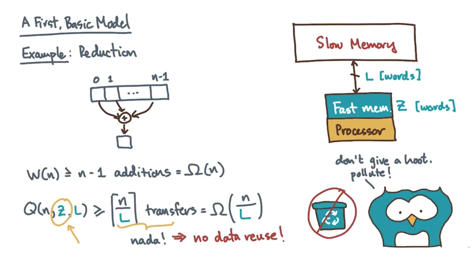
- Can make IO Reductions very specific to note when an IO transfer is happening
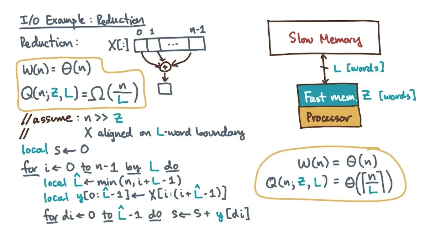
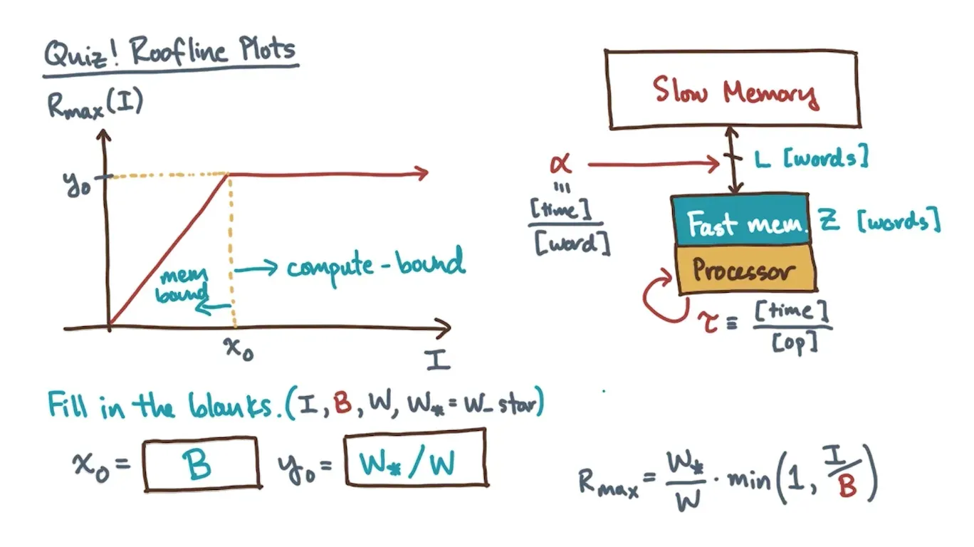
- If W(n) represents work/number of operations on the best sequential algorithm and Q(n, Z, L) measures number of data transfers then the goal is to MAXIMIZE computational intensity ie operations/words
- W(n) / L * Q (n, Z, L)
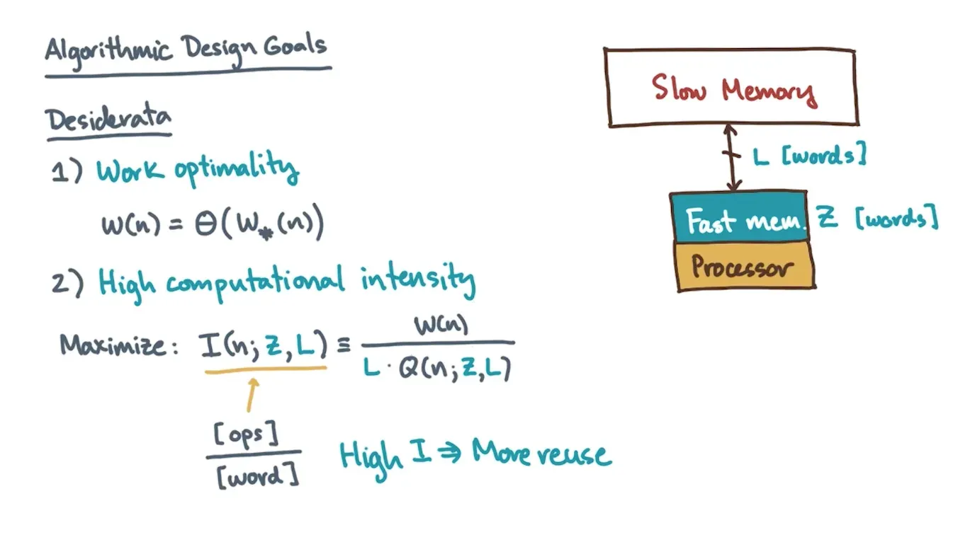
- W(n) / L * Q (n, Z, L)
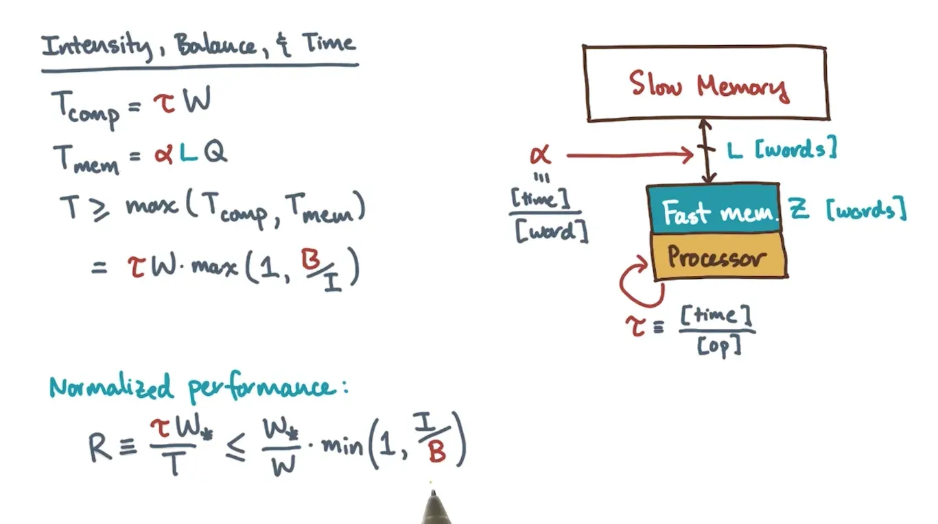
- Lets say processor takes tau time to perform an operation (time/operation) and alpha time to move a word between slow and fast memory (time/word)
- Time to perform compute operations = tau * W(n)
- Time to perform data transfers is alpha * L * Q(n, Z, L)
- Minimum time to execute program is max(time to perform compute operations, time to perform data transfers)
- tau * W(n) * max(1, (alpha/tau) / Intensity)
- computation time * (machine balance/Intensity communication penalty, 1) for inner max
- B = alpha/tau or how many operations execute when move word of data
- simplify to tau * W(n) * max(1, Balance / Intensity) for minimum time to execution
- tau * W(n) * (1 + Balance/Intensity) for maximium time as pay both costs
- tau * W(n) * max(1, (alpha/tau) / Intensity)
- Normalized performance is the best sequential algorithm work/work of your algorithm * min(1, I/B) where higher values are better
- If you do not design an algorithm as optimal as W_star or best sequential algorithm then you will pay a penalty of reduced performance
- If you do not design an algorithm as optimal as W_star or best sequential algorithm then you will pay a penalty of reduced performance
- Compute bound vs memory bound algorithms - make sure to utilize maximum memory
I/O Avoiding Algorithms
- Lower bound of IOs for comparison based sort is (n/L) * log base(Z/L) (n/L)
- Speedups come from the L and log base n/L factors fully utilizing all words when transferring along with fast memory capacity
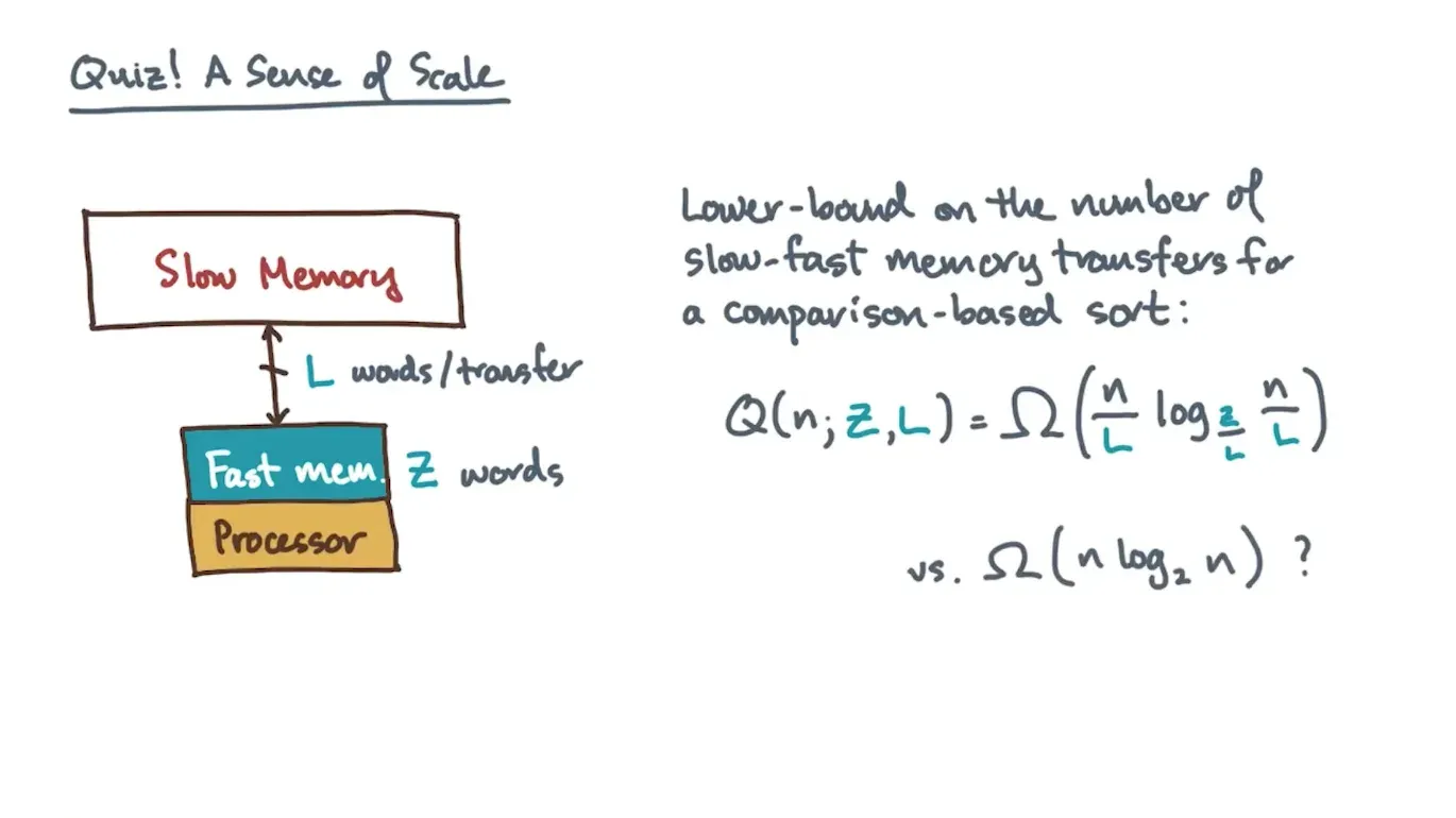
- Speedups come from the L and log base n/L factors fully utilizing all words when transferring along with fast memory capacity
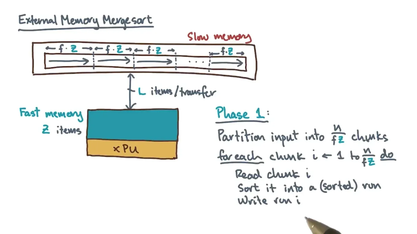
- External memory mergesort takes advantage of fast memory and data transfers
- First split the array into n/Z chunks
- Bring those chunks into fast memory and produce a sorted run
- Afterwards do 1 full pass and merge chunks
- A 2 way merge doesn’t utilize the size of fast memory well ⇒ utilize a multiway/k way merge where (k + 1) * L data fits in fast memory
- Then treat it as an extension of merge k sorted lists
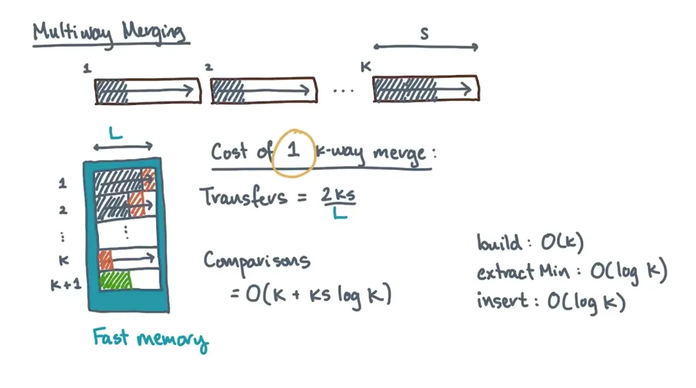
- Then treat it as an extension of merge k sorted lists
Intro to Work-Span Model
- Parallel algorithms can be represented in a DAG where nodes are units of work and edges indicate dependencies where outgoing edge node cannot start until all predecessors complete
- Algorithm creates a DAG, multi-core machine figures out how to map it to cores
- Start at root node for DAG, assign it to a processor, and once dependencies are satisfied for node, can assign it to a process to run, repeat until end
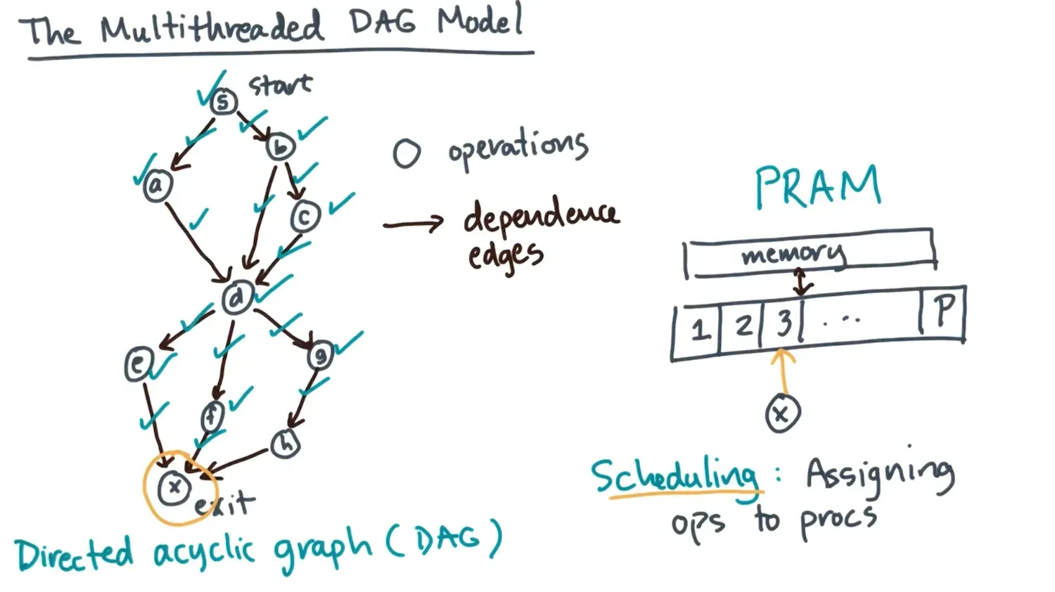
- For adding all elements in a list, every element must be loaded and then the addition depends on the loads
- Can represent this sequentially or tree based o(n) time vs o(logn) time
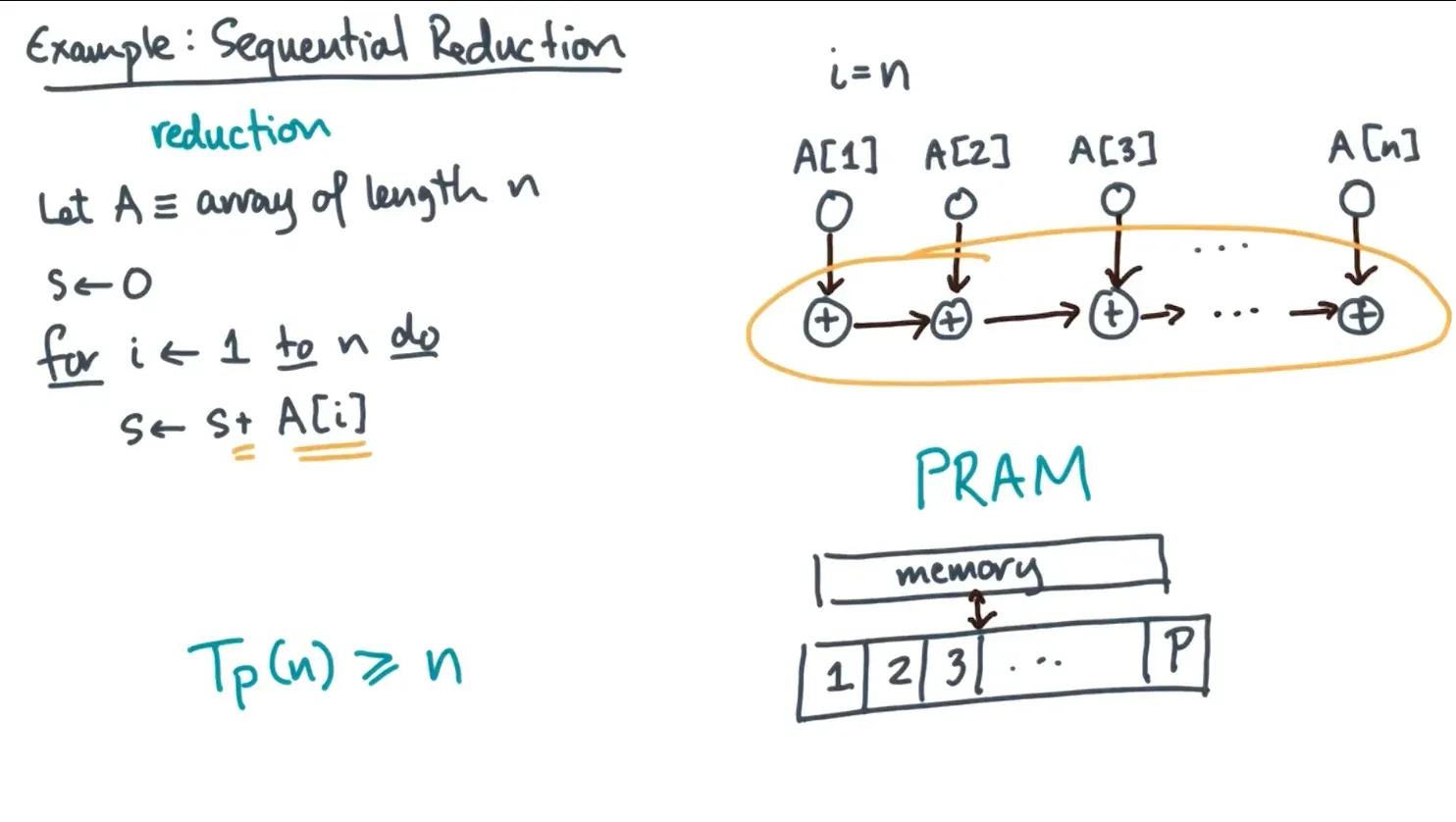
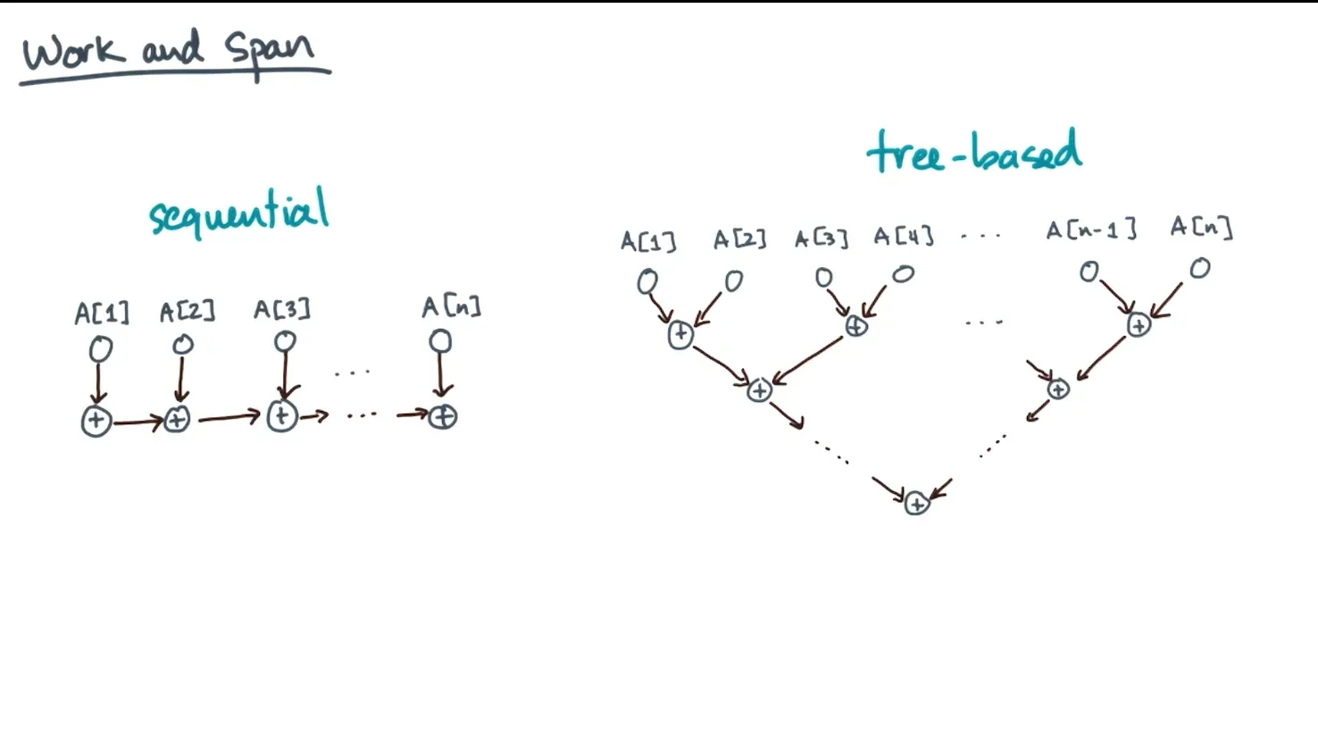
- Can represent this sequentially or tree based o(n) time vs o(logn) time
- How do we know if the DAG we created is performant? ⇒ Work Span Model
- Work is the number of vertices and the time it would take if 1 processor executed DAG
- Span is the number of vertices on critical path and the time if we had infinite processors that executed the DAG
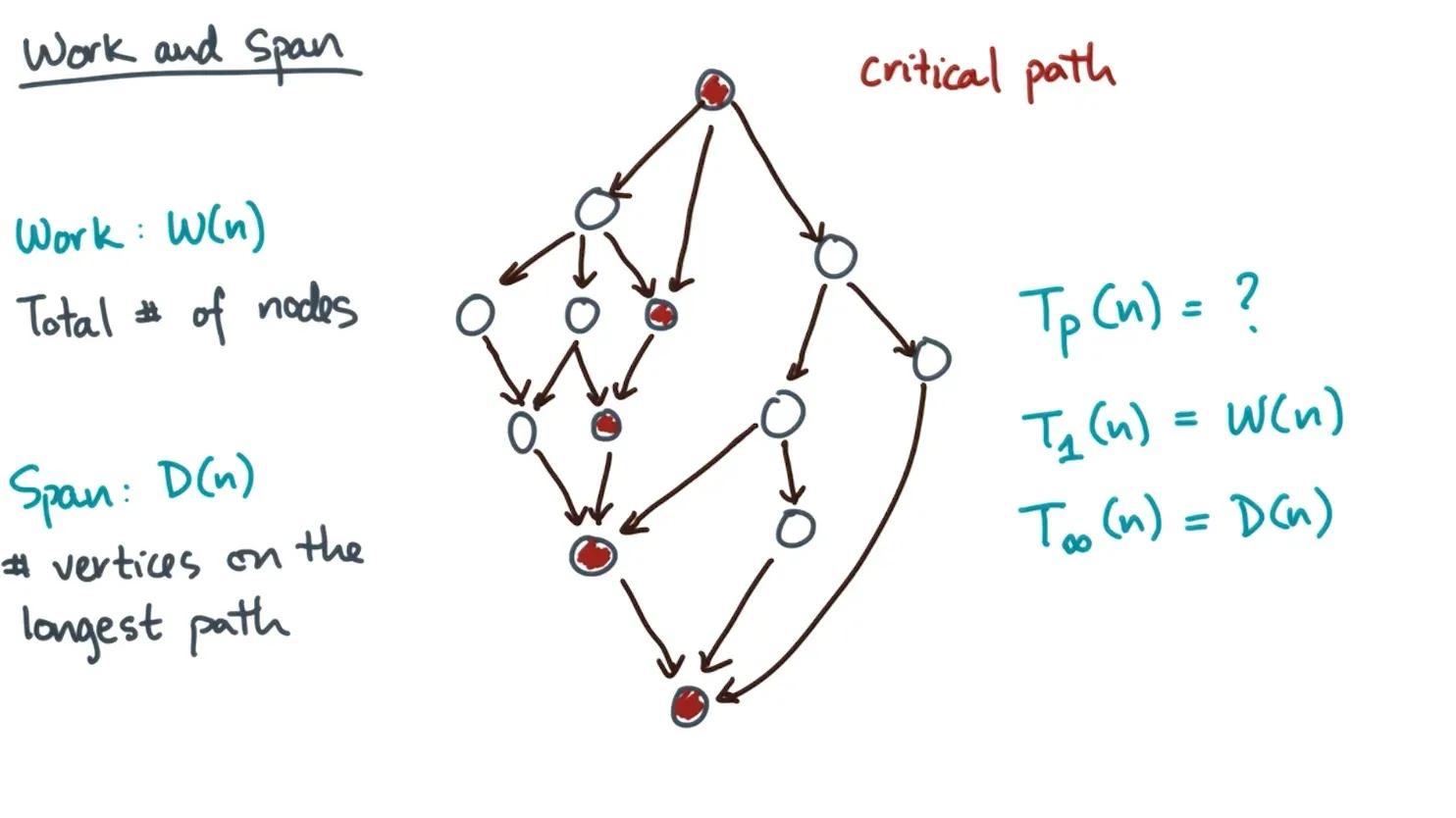
- The average available parallelism ie how many processors should we allocate for this parallel algorithm is Work/Span
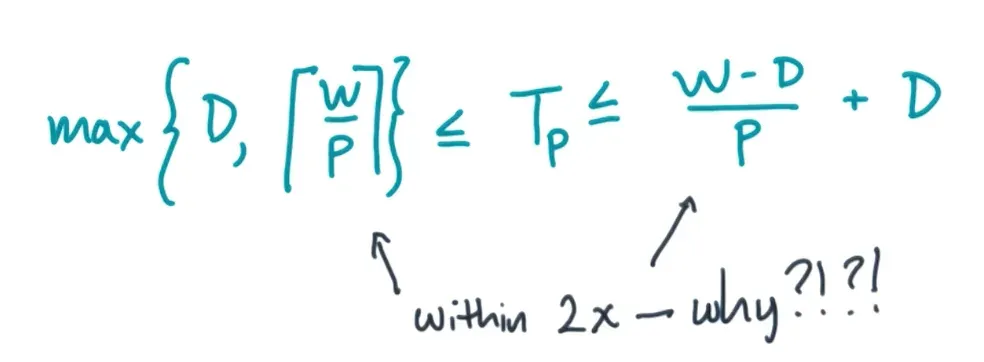
- 2 lower bounds we can use is traversing all of Span or D(n) or if there is no critical path then assigning p processors to Work or W(n) ⇒ take max of both for a lower bound
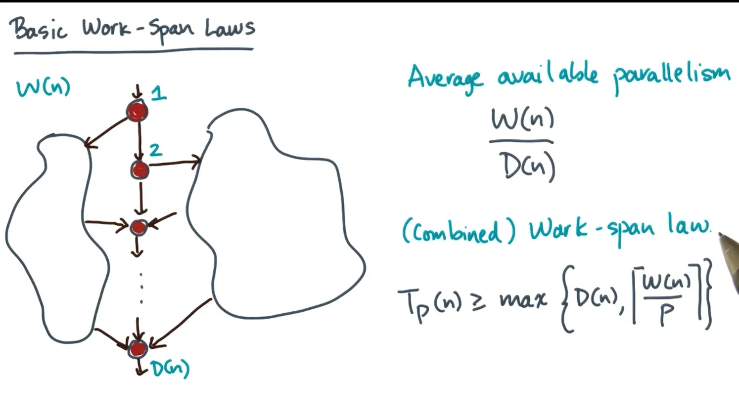
- 2 lower bounds we can use is traversing all of Span or D(n) or if there is no critical path then assigning p processors to Work or W(n) ⇒ take max of both for a lower bound
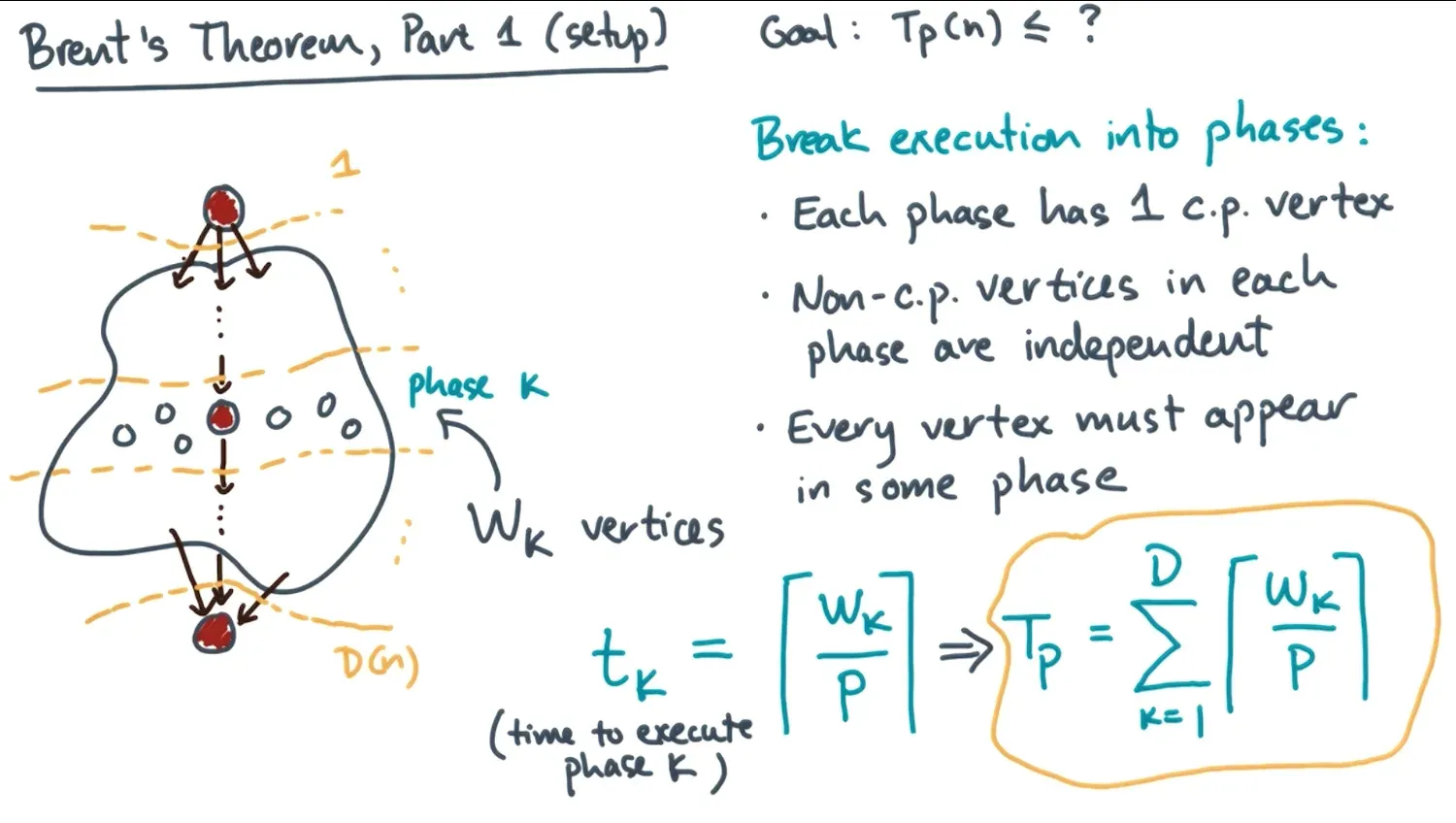
- We can get upper bound to execute this DAG using Brent’s theorem
- First break the execution into phases
- Every phase has a critical path vertex
- Every non critical path vertex are independent from each other - no shared connected edges between them
- Every vertex appears in some phase
- TIme to execute all levels from k = 1 to D is ceil(Wk/p)
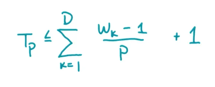
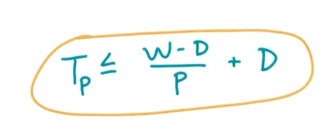
- Now apply algebraic theorem to convert ceiling to floor and now Brents theorem states that the upper bound is execution of the critical path + execution of everything else divided up into p processors
- First break the execution into phases
- Lower and upper bound are within a 2x bound
- How do we know if a parallel algorithm is good
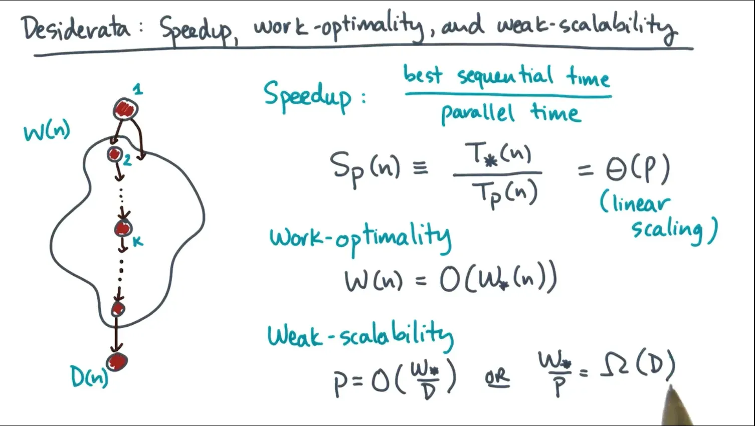
- First lets get speedup by getting the best sequential time / parallel time
- Now ideally with p processors we want a O(p) speedup
- Work of the best parallel algorithm should match work of the best sequential algorithm
- Work per processor should grow as the span grows
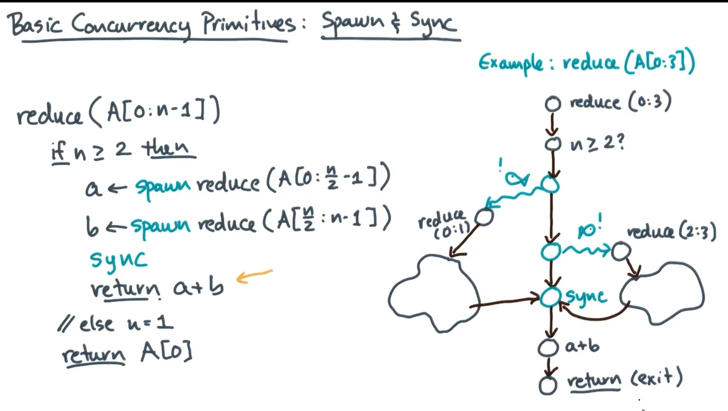
- For concurrency purposes, spawn generates a new independent unit of work and sync waits for all spawns only in the same stack frame
- If no sync provided, then an implicit sync will be provided (probably wont be correct since values computed is before sync so may not be computed already)
- If no sync provided, then an implicit sync will be provided (probably wont be correct since values computed is before sync so may not be computed already)
- Work and Span can be analyzed the same was as in algorithms
- Solve either with recurrence tree or master theorem
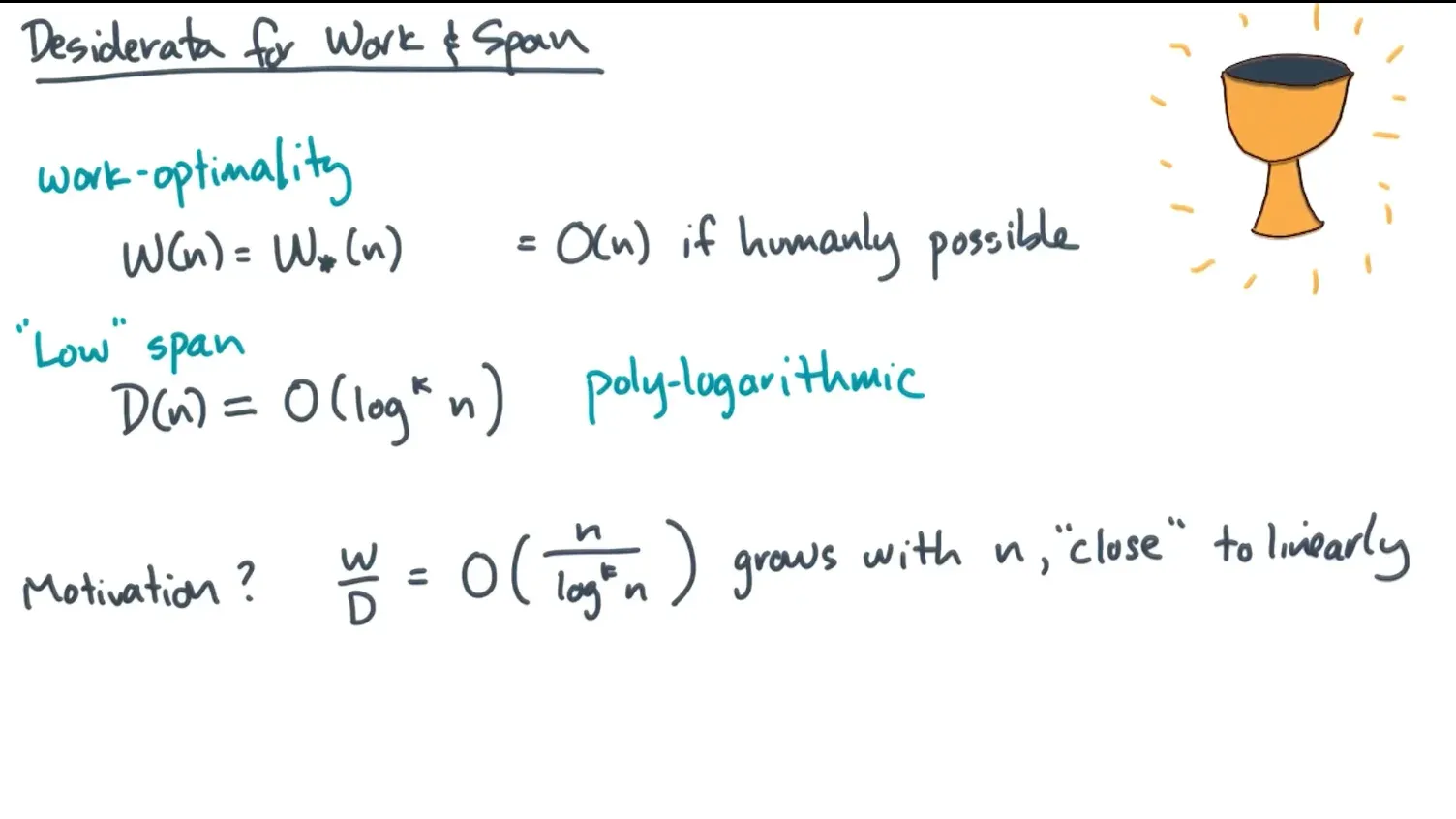
- Ideally want work to be linear or below and span to be polylogarithmic/divided and conquered so that it grows with n linearly
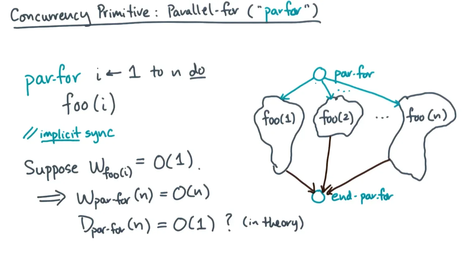
- Another concurrency primitive is parallel for which makes all iterations of for loop independent
- Span here is O(n) with for loop as the actual for loop creates n nodes
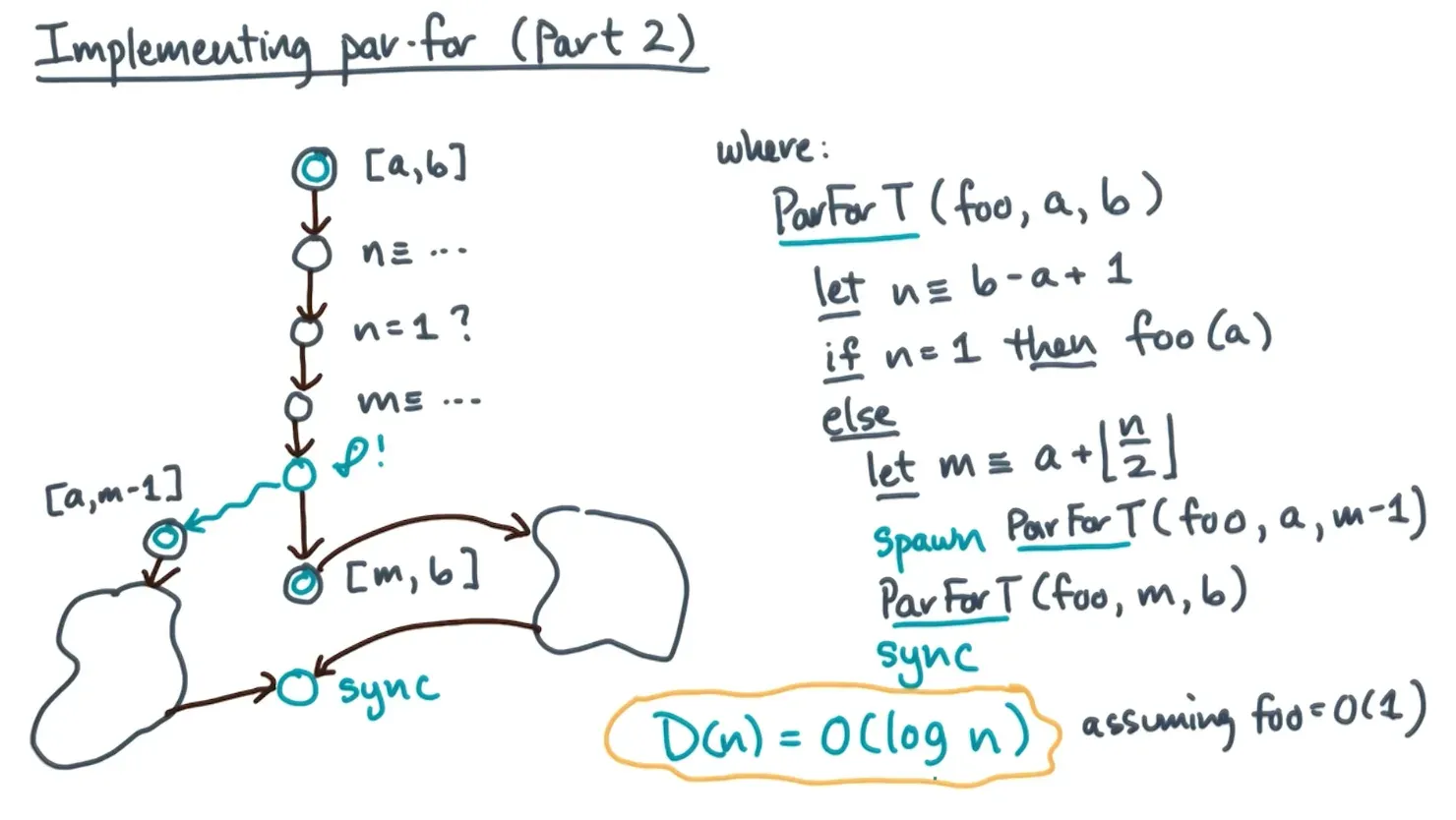
- Can divide and conquer with spawn/sync for O(logn) span
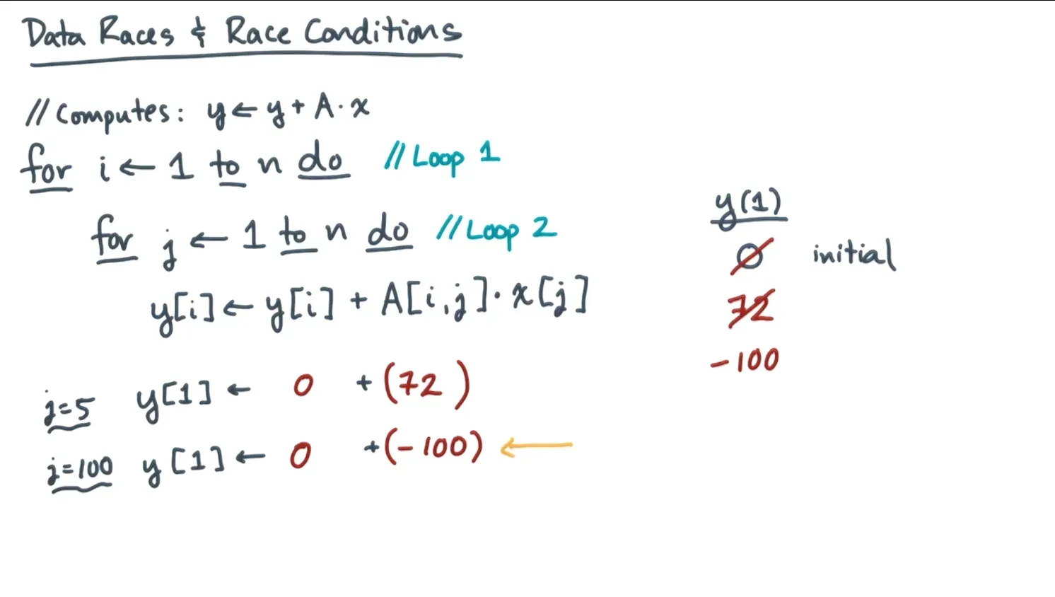
- Need to make sure that parallelization doesn’t result in race conditions/data races
Comparison Based Sorting
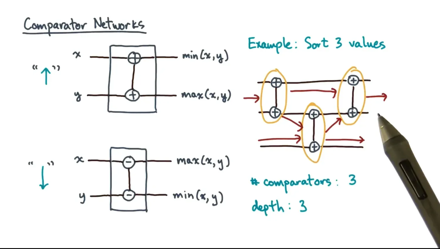
- Can sort elements via comparator networks (think in hardware)
- Bitonic sequences are sequences that first increase and then decrease OR if it holds for a circular shift of the sequence (last element connects to first element)
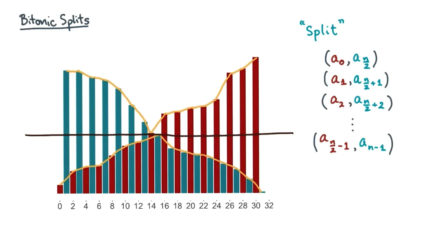
- Imagine taking a bitonic sequence and then splitting it in half and for every sequential element of every half, assign pairs (a0, an/2)…
- If we take the min of every element from the pairs we have a bitonic subsequence
- If we take the max of every element from the pairs we have a bitonic subsequence
- All max elements of the resulting bitonic subsequence are greater than the min elements of the bitonic subsequence ⇒ divide and conquer bitonic split sorting
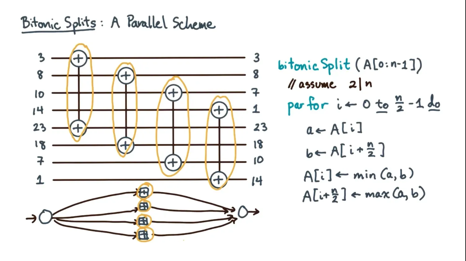
- Can run bitonic splits in parallel
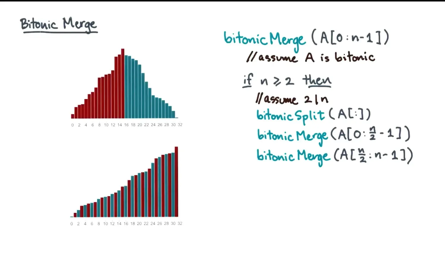
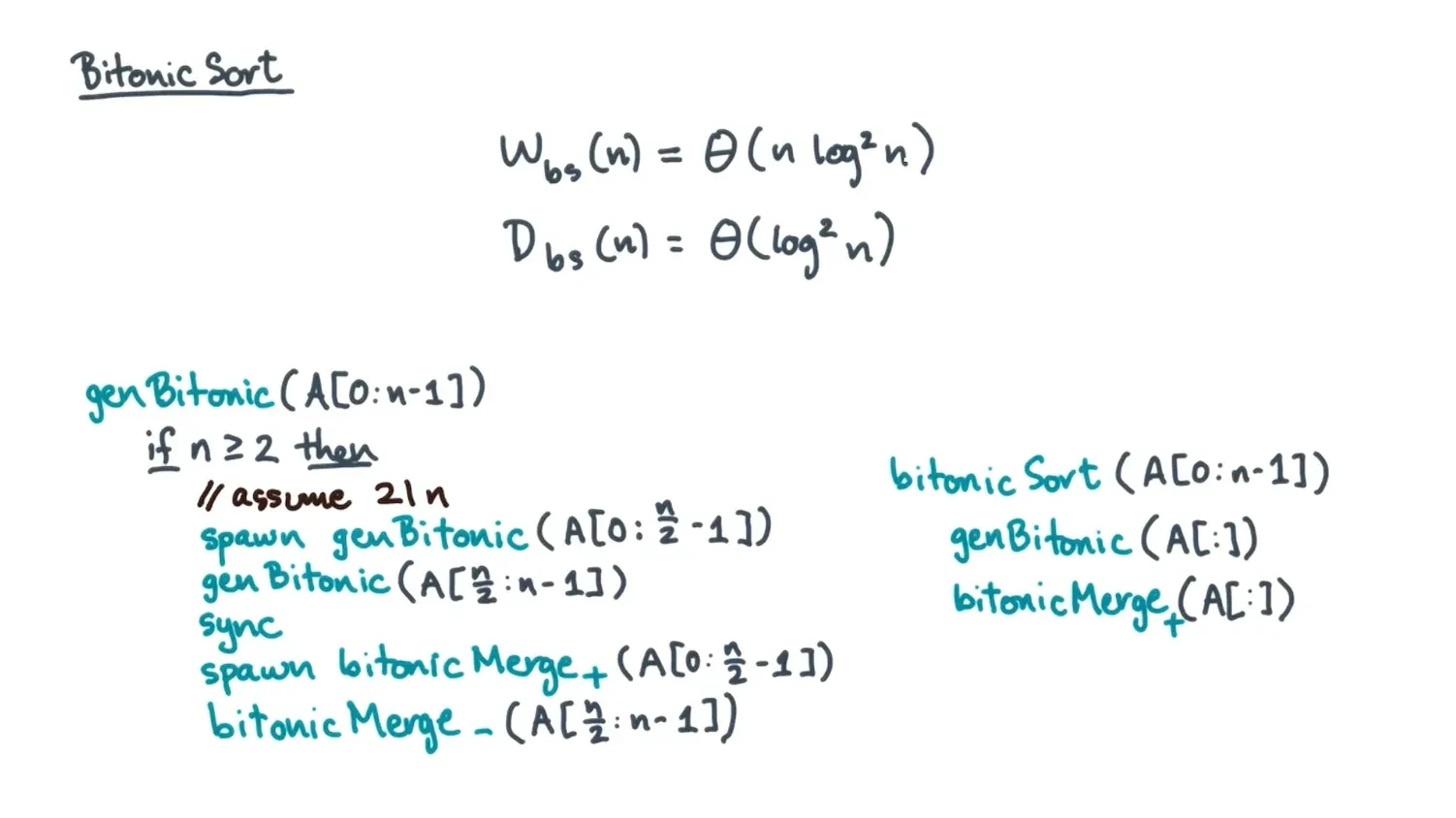
- Imagine taking a bitonic sequence and then splitting it in half and for every sequential element of every half, assign pairs (a0, an/2)…
Scans and List Ranking
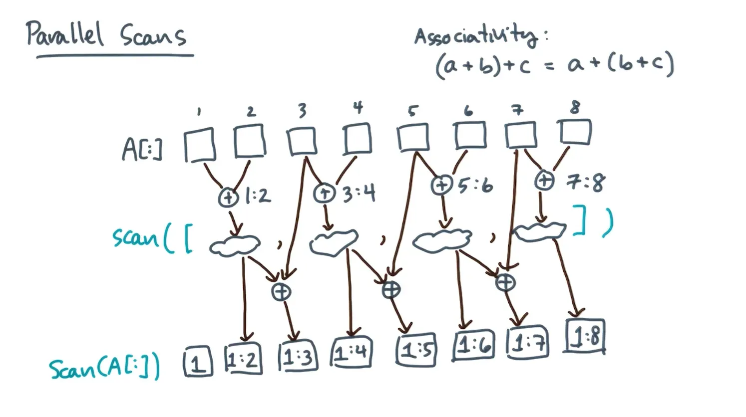
- Prefix sum is cumulative sum from i = 1 to a given k index
- Can generalize this to other operations ie add scan, product scan, add scan where all scans perform the specified operator on a prefix
- We know that (a + b) + c = a + (b + c) by associativity so why not apply this to prefix sums
- Can we use divide and conquer?
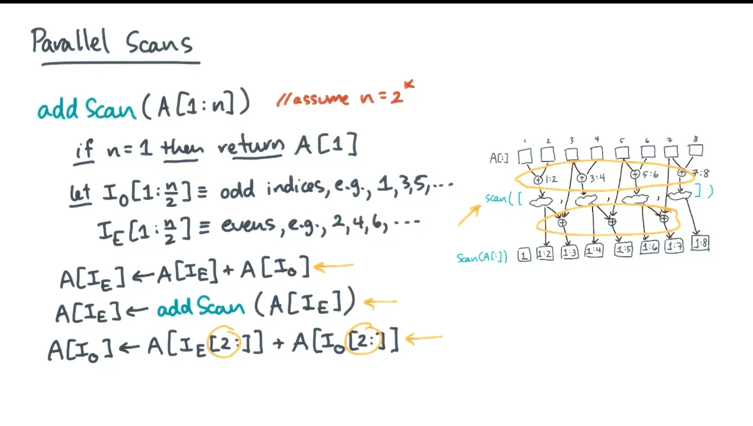
- We add prefixes of even elements by combining arrays of length 2
- Then we use a special scan algorithm to get the prefix sum of all even elements
- Now that we have all the even elements, we just need to add currOdd[i] + prefixEven[i] to get all the odd elements
- O(2n) work instead of O(n) ~ do we need to pay something to achieve parallelism?
- O(log^2n) as logn parallel for loop + recursive function on half the elements
- Can we use divide and conquer?
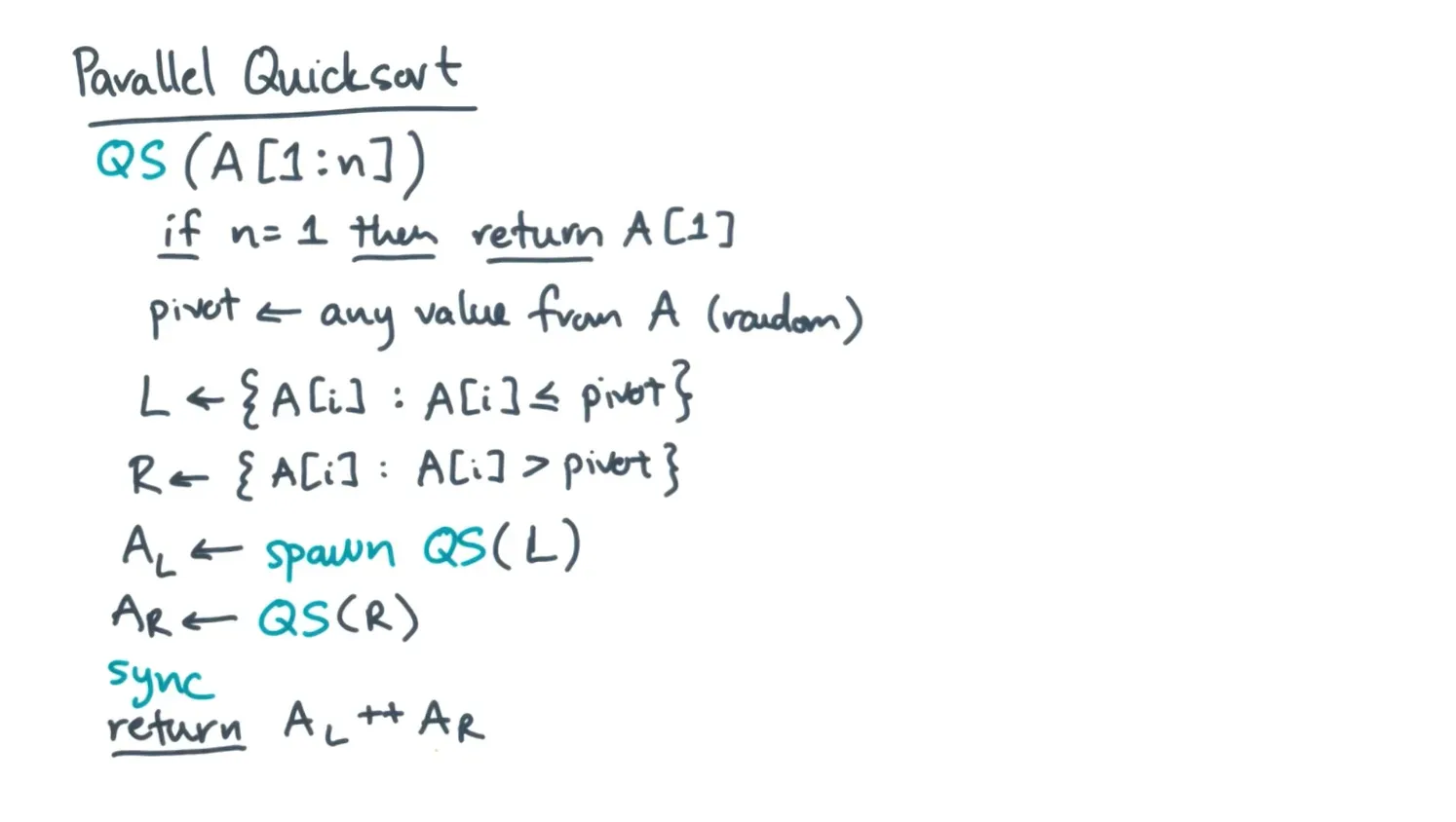
- We can parallelize quick sort interestingly enough with prefix sums
- We would like to partition in parallel
- Don’t by default parallelize the partition for loop → would lead to race conditions since how can we deal with 2 elements being partitioned at once w/o locks
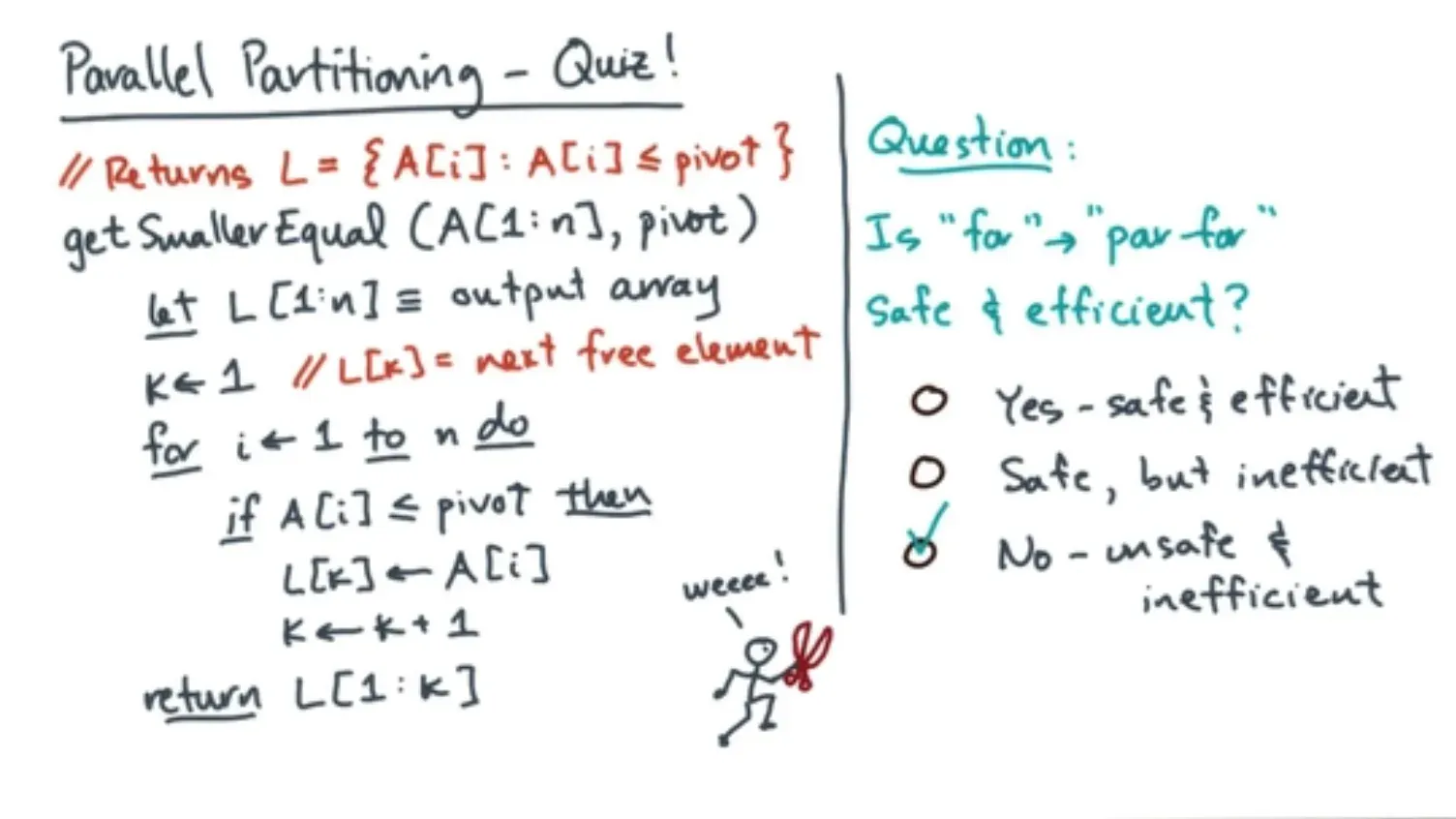
- Instead maintain a boolean array of elements ≤ pivot, perform an addition scan, and now we have
- The number of elements before/after a given pivot
- The unique consecutive indices of elements before/after a given pivot that can be parallel written to output
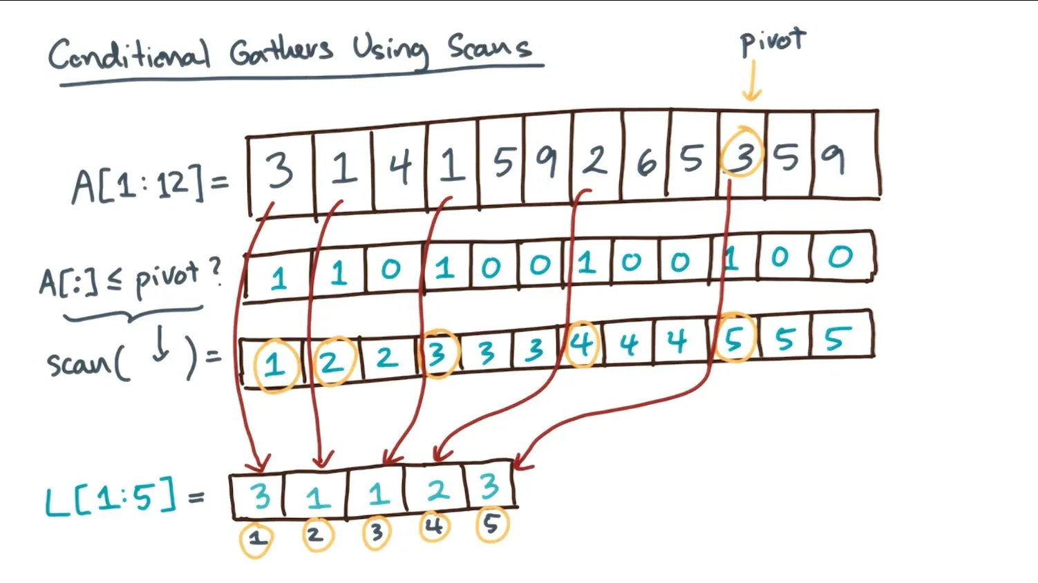
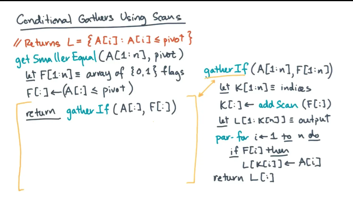
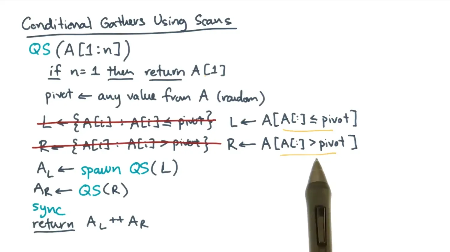
- We would like to partition in parallel
- What if we want to perform scans on segments of the array given an array of flags where True represents the start of a segment?
- We can take in pairs of tuples, check if the latter is false, and then return a new tuple that is the sum of the tuples + an OR of the flags in order not to merge separate segments
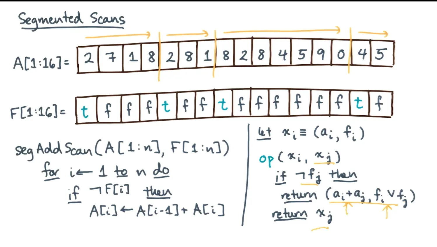
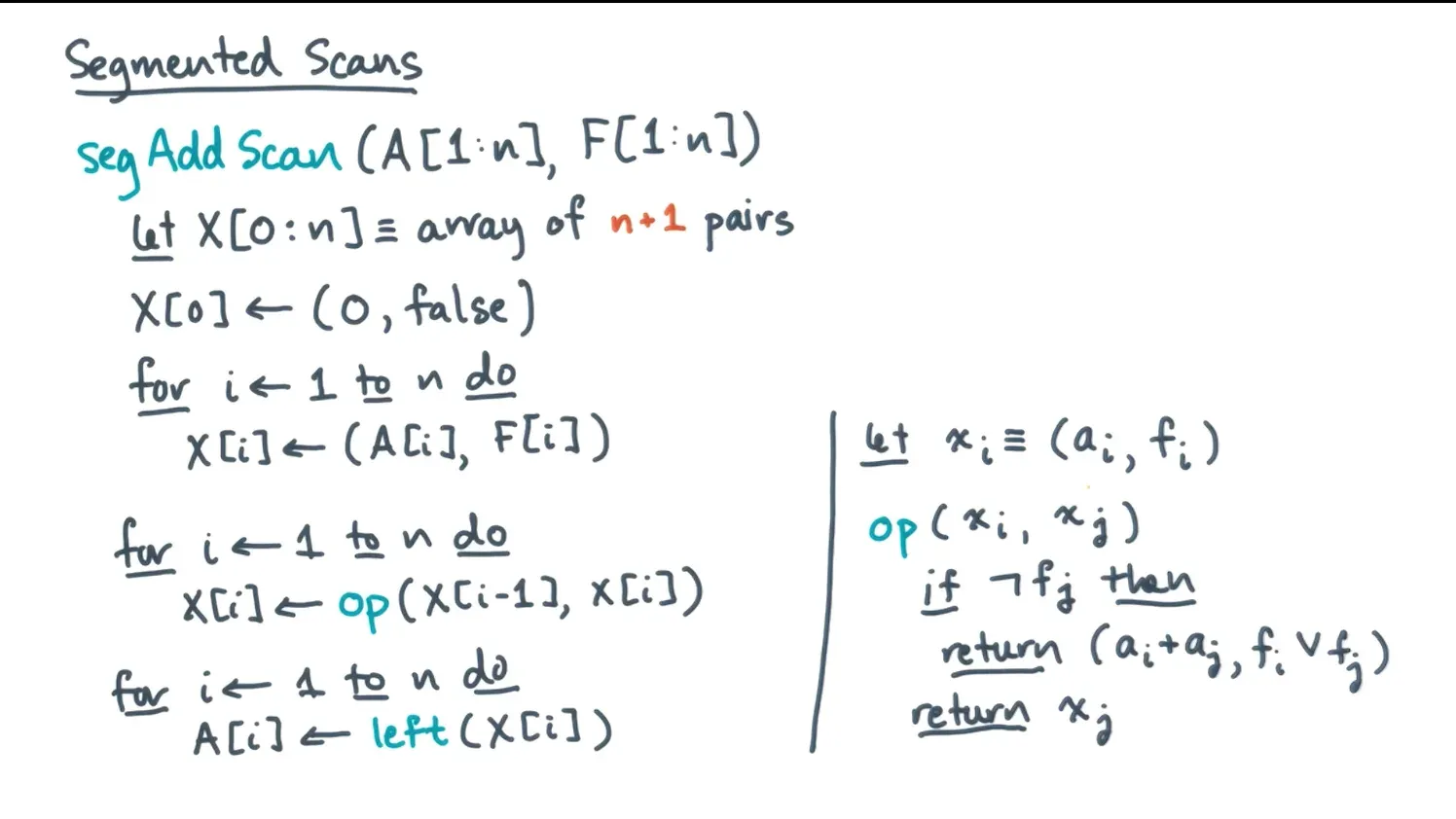
- We can take in pairs of tuples, check if the latter is false, and then return a new tuple that is the sum of the tuples + an OR of the flags in order not to merge separate segments
- List ranking involves getting the distance of every node from the head which is simple sequentially but how to parallelize?
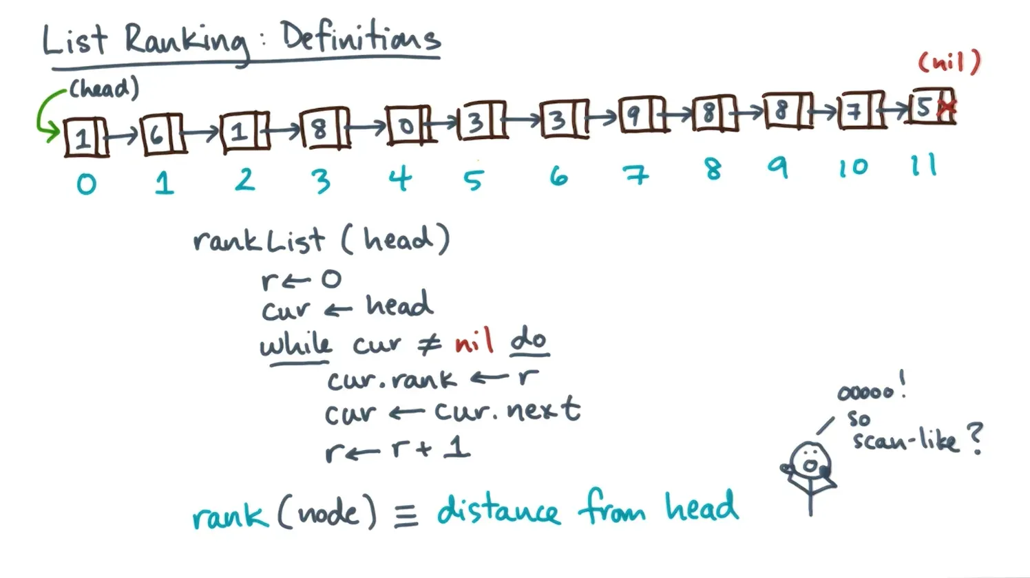
- Why not store the list as an array where V[id] is the value of the list at that given id and N[i] is the value of the next nodes id of that list
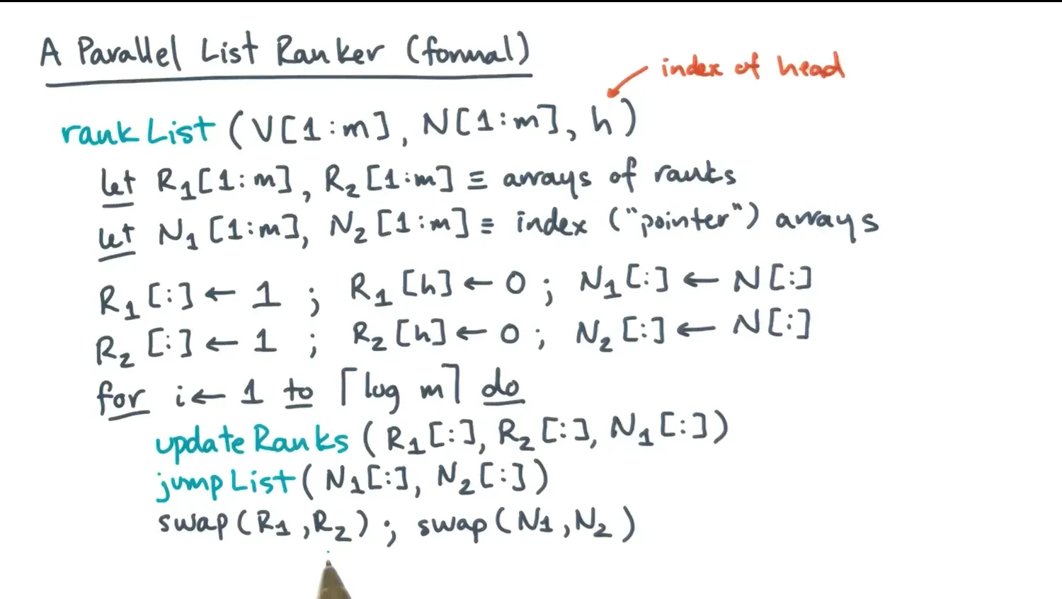
- Wyllies algorithm has nlogn work and log^2n span by utilizing a divide and conquer and scan approach
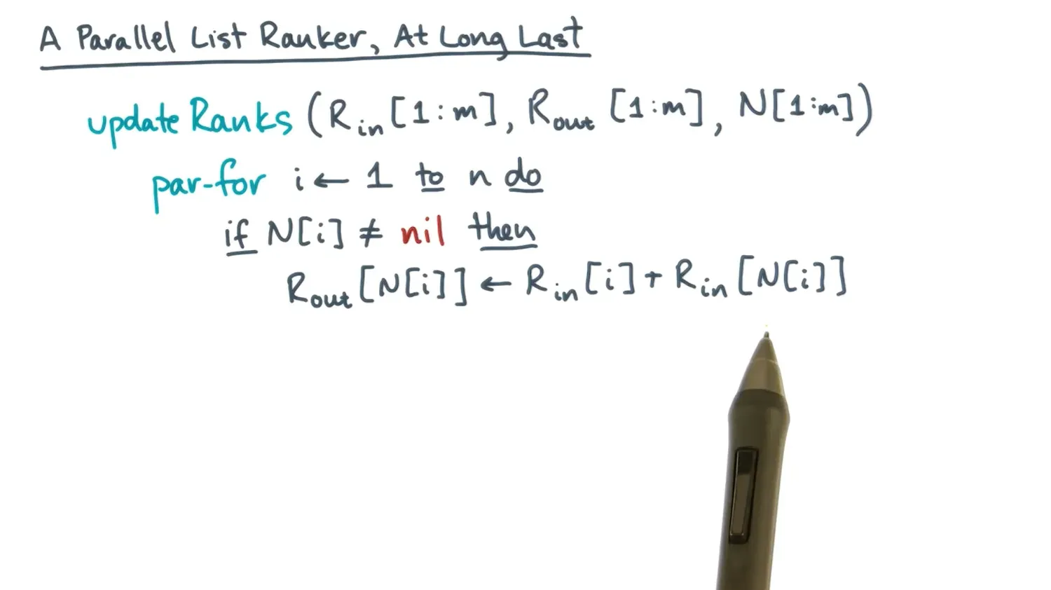
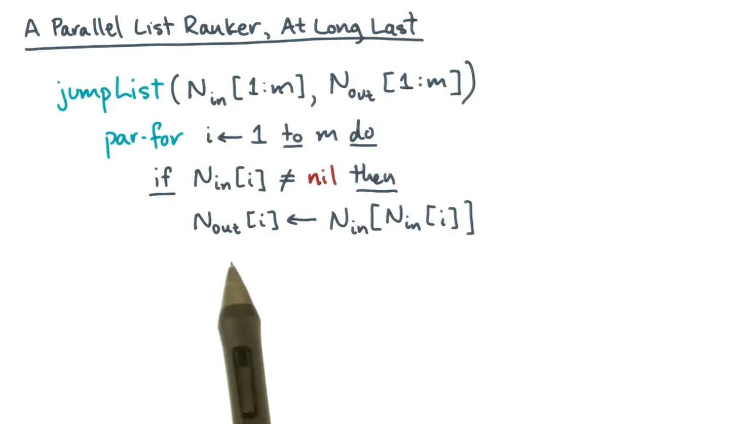
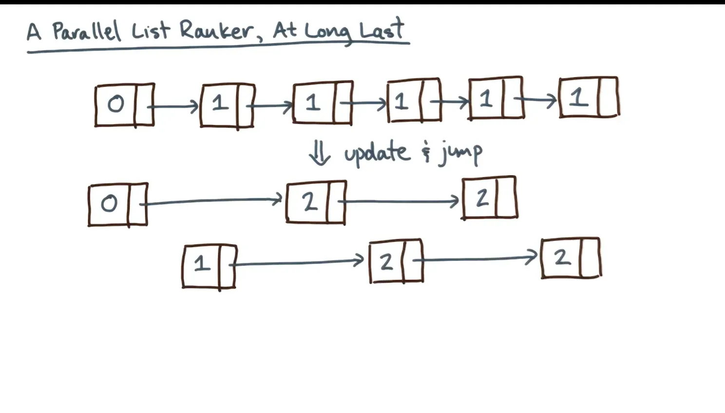
- For ceil(log(m)) iterations, update the lists by adding the prev nodes value to its next nodes value + jump lists by setting every lists next node to the next next node
- Updating ranks and jump lists are parallelizable with a for loop
Intro to OpenMP
Scaling on GPUs
Tree Computations
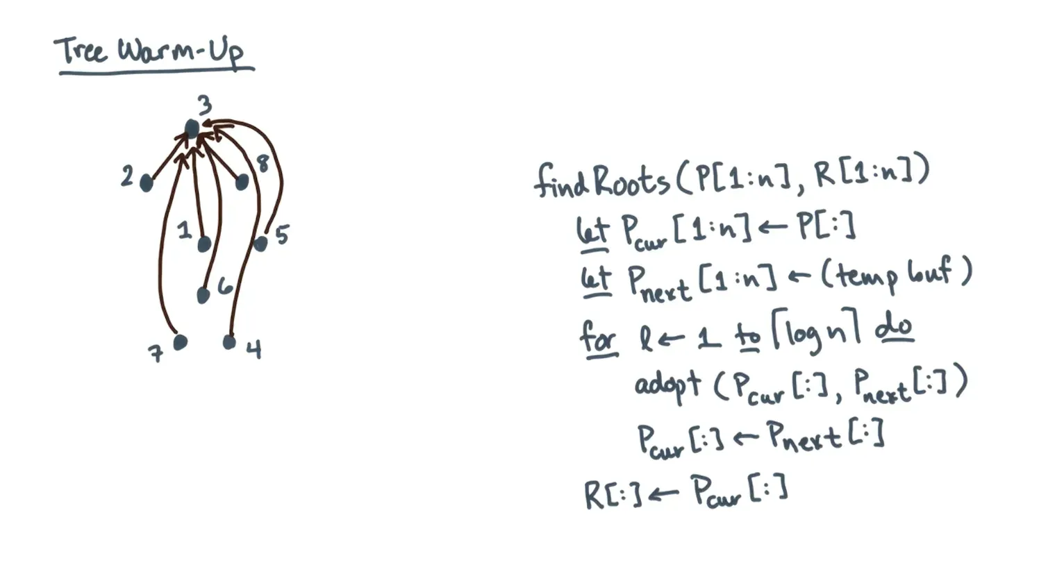
- Can store trees in an array where parent[i] is the parent of node i and p[i] = 0 is the root node
- A simple way to find a root is to pick a node and follow the parent pointer until we reach the root - not parallel
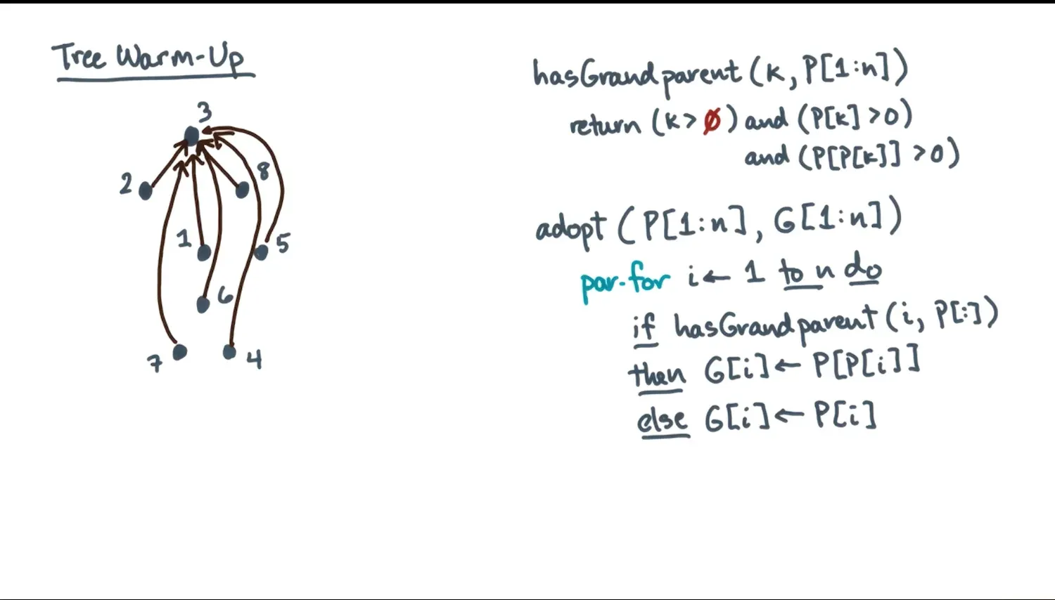
- To run this in parallel, for log n levels, we set the current nodes parent to its grandparent so all nodes will point to the root (we reduce the size of the tree by half every time) + parallel adopt point jumping
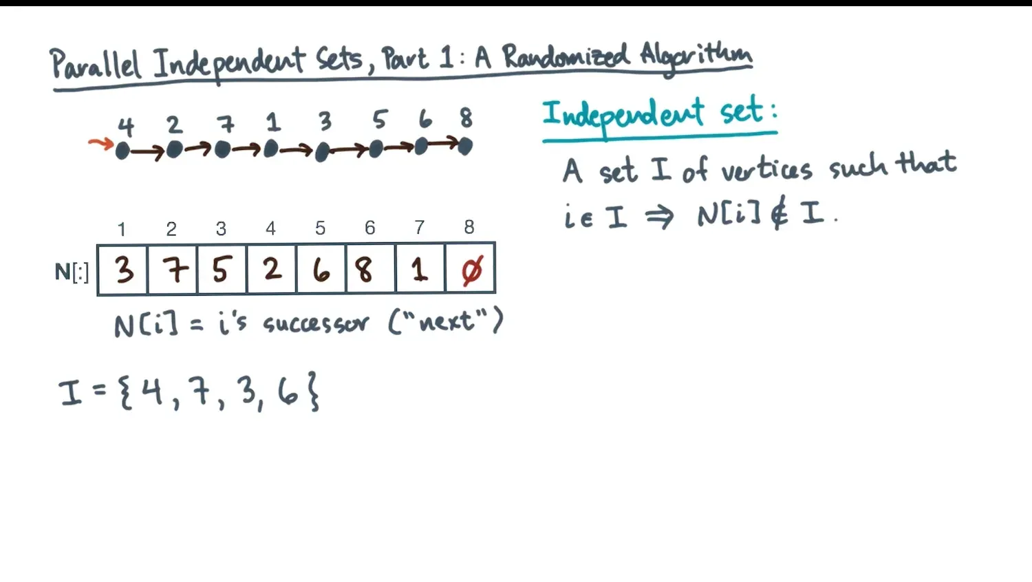
- How would we generate independent sets or vertices where for every node i, its successor is not present
- Sequentially loop over nodes and don’t add its successor
- But how to do this in parallel, for every node i in parallel, it is isolated and independent from other nodes so we don’t know if we can add it
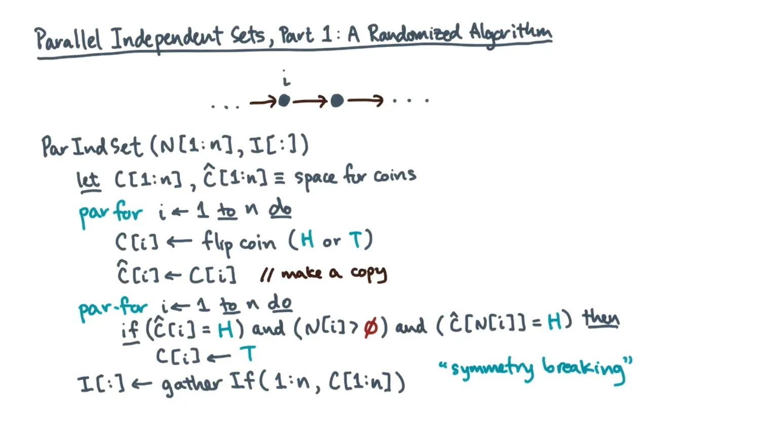
- Use coin flips to assign nodes
- For every node in parallel flip a coin - heads included and tails excluded
- For every node in parallel if successor node is a head, then change current node to a tail
- However only 1/4th of the nodes make it into this independent set (out of ht tt th hh ⇒ ht is only valid)
- Once we have flipped coins, remove vertices from independent set, push the removed vertices temp ranks to the next nodes, and jump prev pointers to next pointers and repeat log(log(n)) times
- Use coin flips to assign nodes
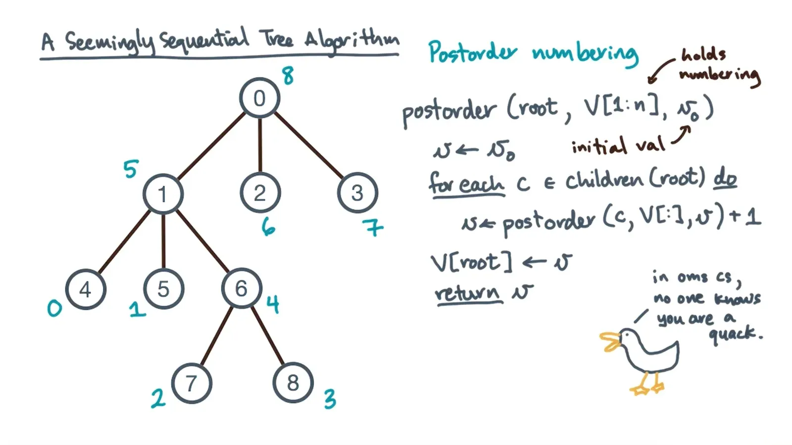
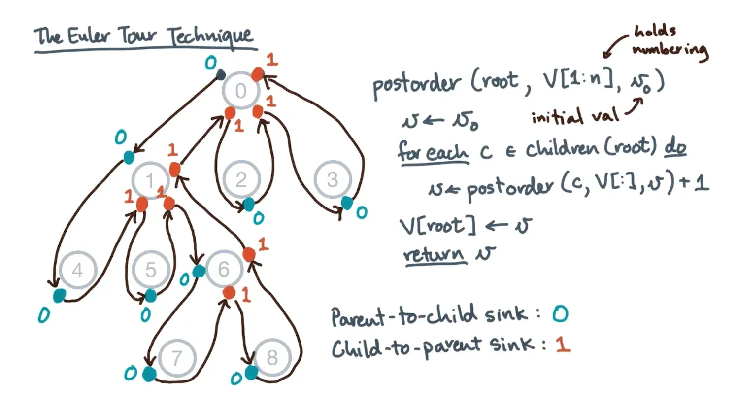
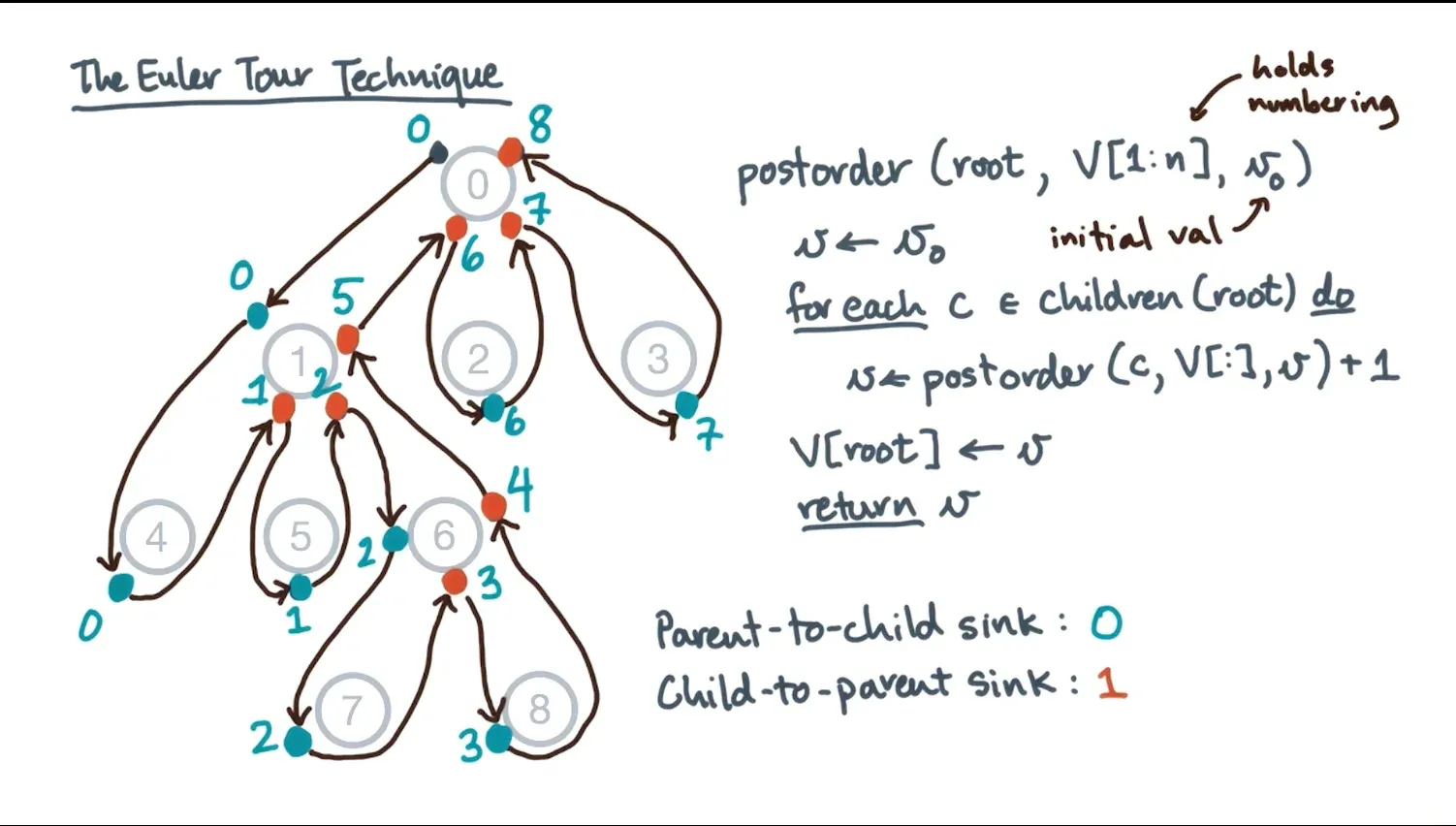
- Postorder traversal of a tree assigns values of every node from child to parent to root - looks parallel but similar to list ranking
- What if we made the tree eulerian ie turn it into a list?
- Then get the Euler circuit here or the path that uses every edge once
- For any sink nodes (parent to child nodes), mark them with a 0
- For any reverse sink nodes (child to parent) nodes ie coming back from recursive call, add 1 to them
- Then do prefix scan by following Euler circuit
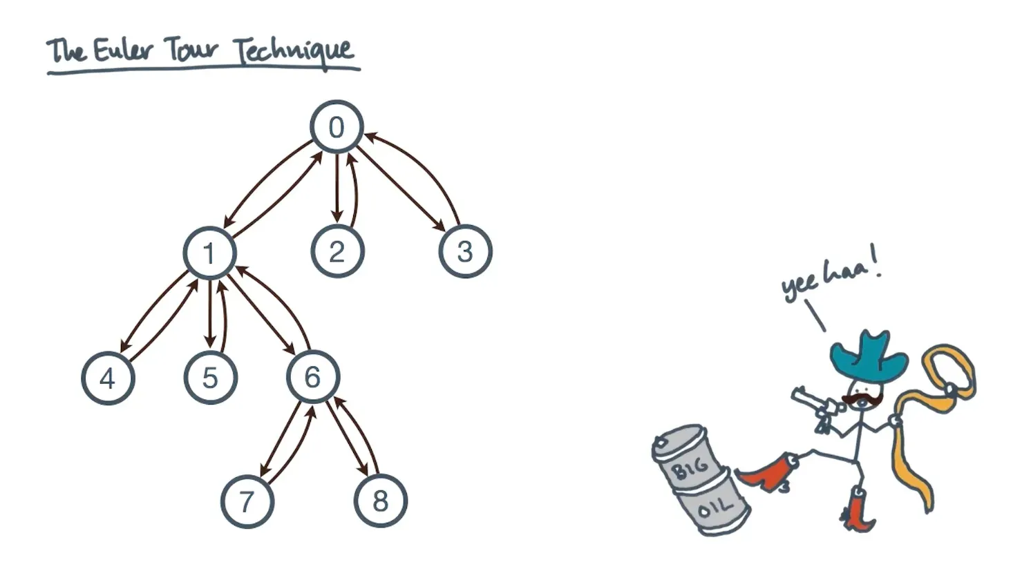
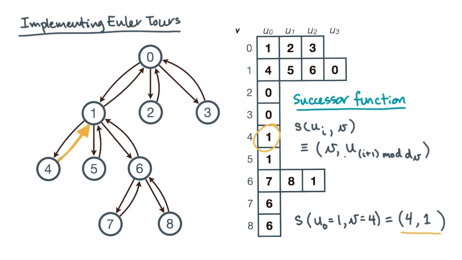
- Can implement Euler tours with an adjacency list and a successor function with extra edges to traverse easily
Intro to Distributed Memory Models
- For massive amounts of data, you want to use distributed memory models
- Overview of distributed memory and rules
- Time to send a message is latency + inverse bandwidth * n messages
- If multiple messages happen over the same link then k way congestion on the bandwidth
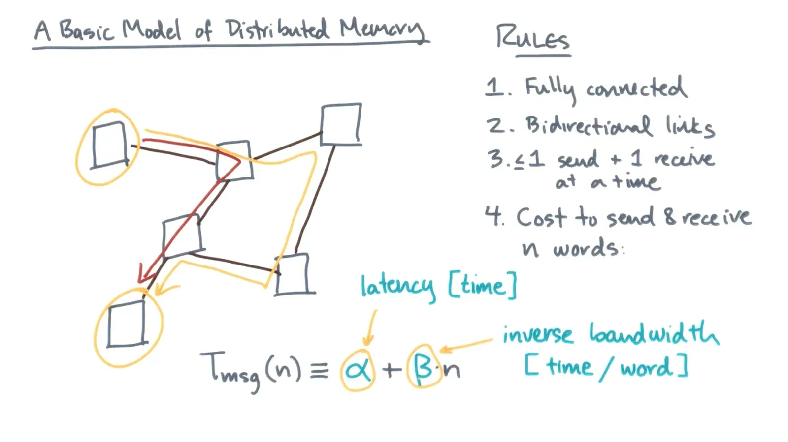
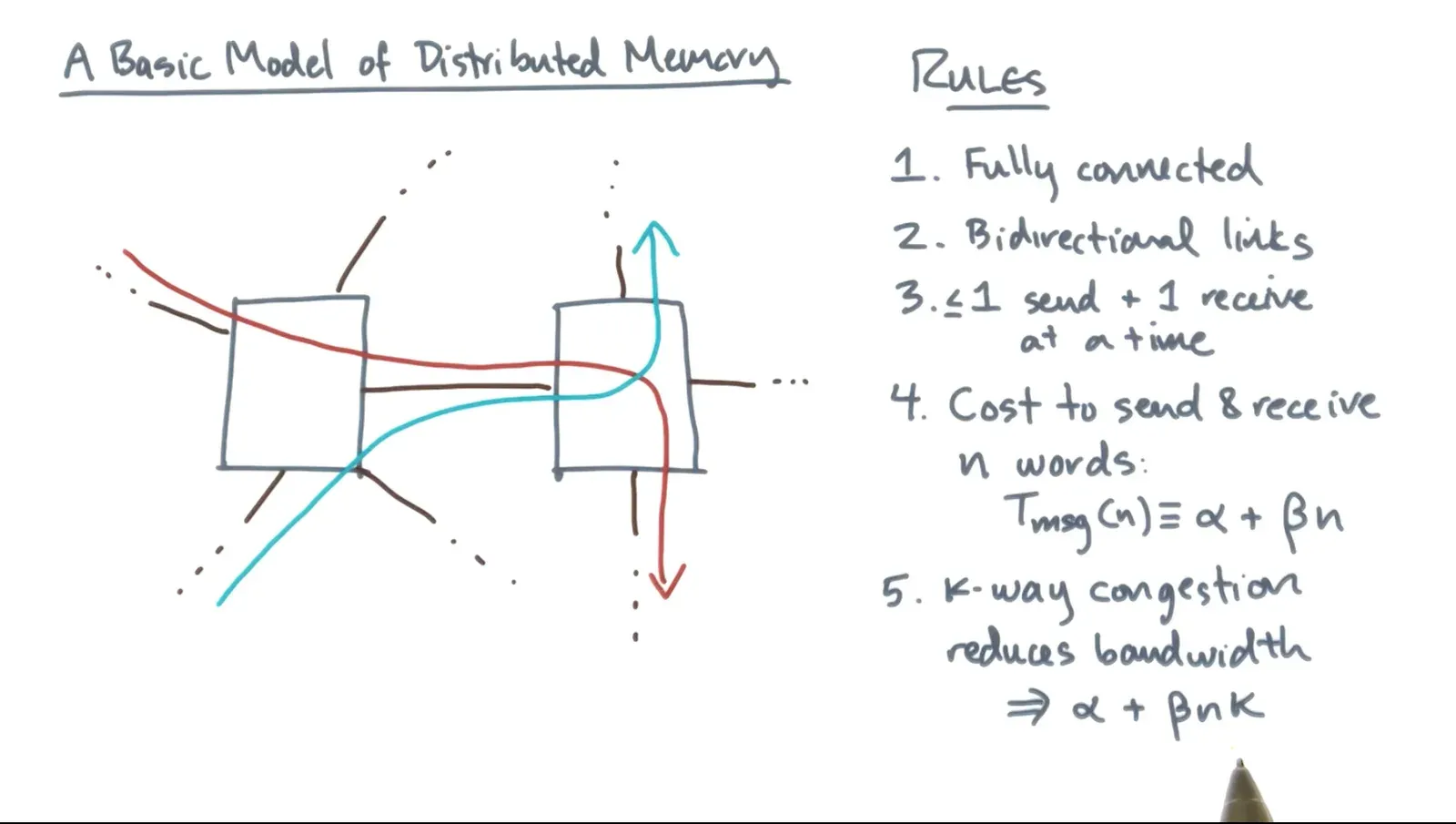
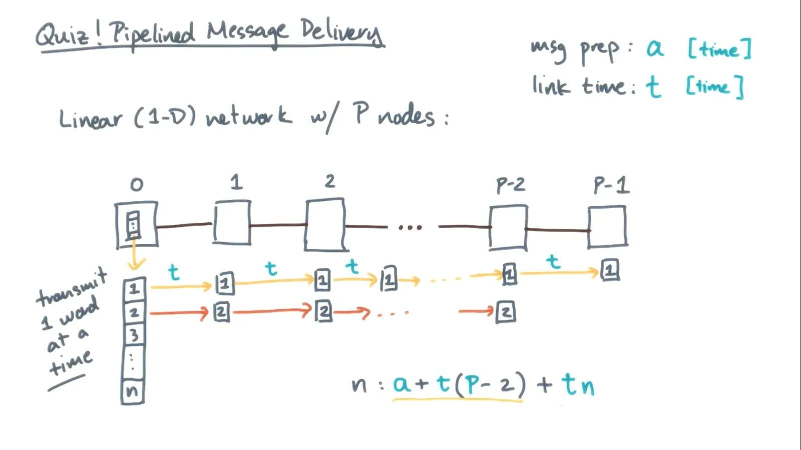
- The distributed memory model has a couple of primitives
- It is SPMD (Single program multiple data) so all processors run the exact same program but had a unique id (rank)
- Can send messages asynchronously
- Can recieve messages asynchronously
- Can wait on messages and block thread either on 1 handle or all handles
- Every send must have a matching recieve
- The buffer is able to be reused after a recieve but not a send (what if we have to wait for the recieve to initialize on the other process?)
- Reductions involve the odd elements of the set of nodes sending their messages over (look at least significant bit to determine)
- Can reduce vectors to 1 root and the opposite of this is broadcasting the vector to all processors
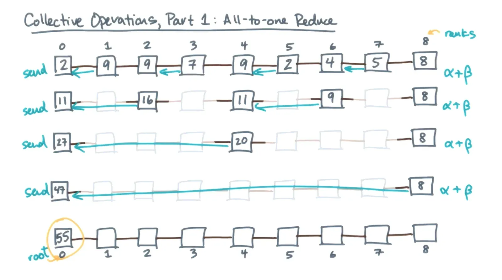
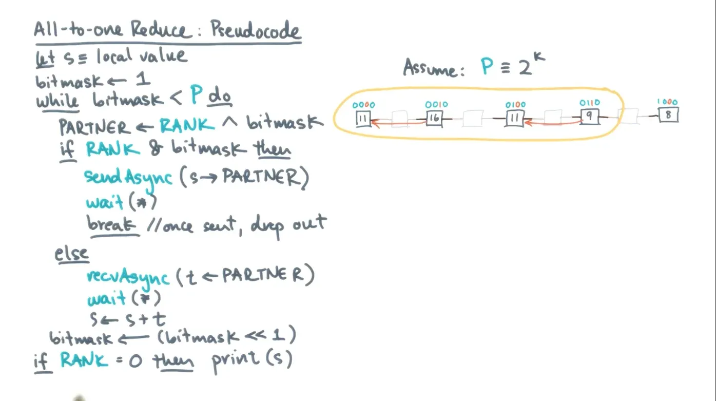
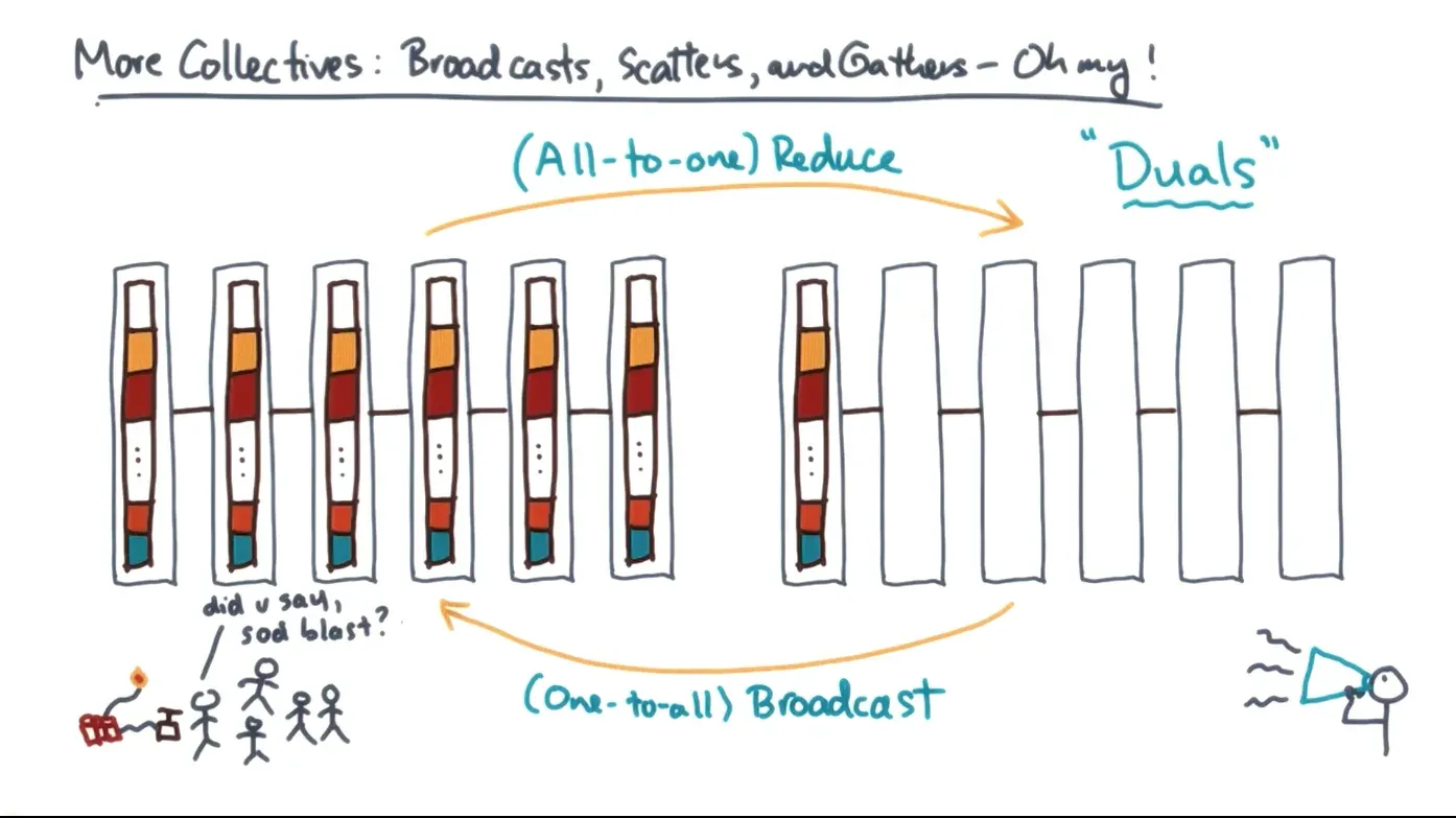
- Can reduce vectors to 1 root and the opposite of this is broadcasting the vector to all processors
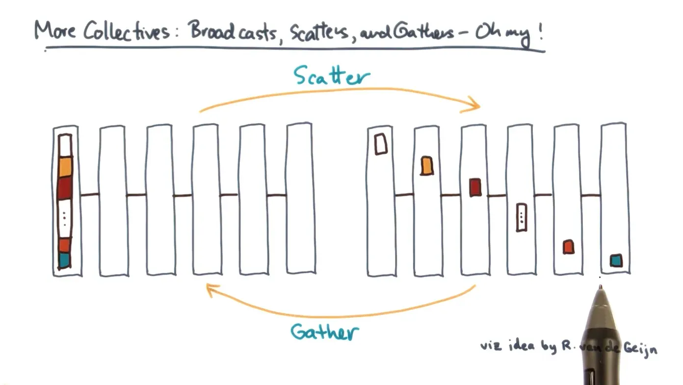
- Scatter takes a vector from the root and places data intermittently in every other processor and gather does the opposite
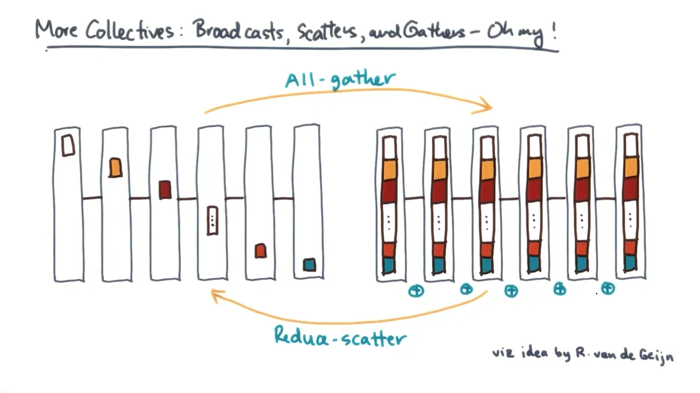
- All gather takes the pieces of data from each nodes and builds up the vector for every other node and reduce scatter is the opposite
Topology
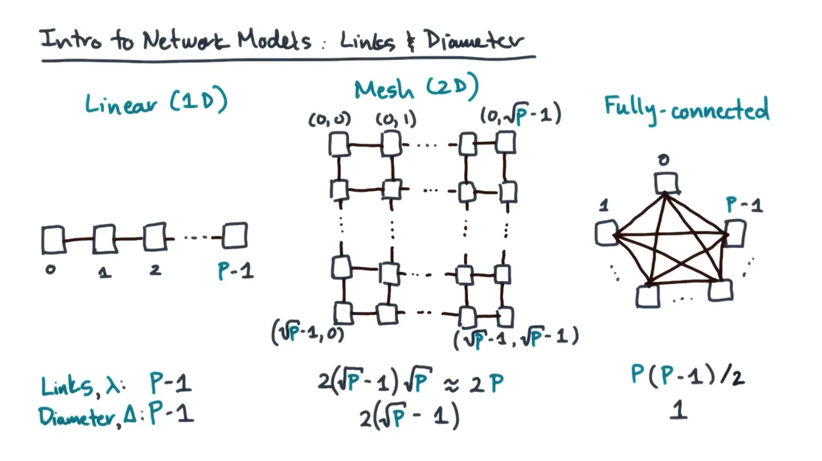
- Networks go from linear to 2D mesh and fully connected networks
- The more links/connections between nodes, the more expensive initial setup is
- The shorter the diameter (longest shortest path) the shorter it takes to send messages
- Bisection width is the minimum number of links to cut the network in half
- Important for all to all collective where every node wants to send data to every other nodes so data will travel over the bisection
- Bisection bandwidth is the bisection width * bisection bandwidth
- Many different network topologies which affect performance
- Trees have scalable links and diameter but poor bisection as only 1 way to transfer
- Make fat tree by adding more links the higher level you go
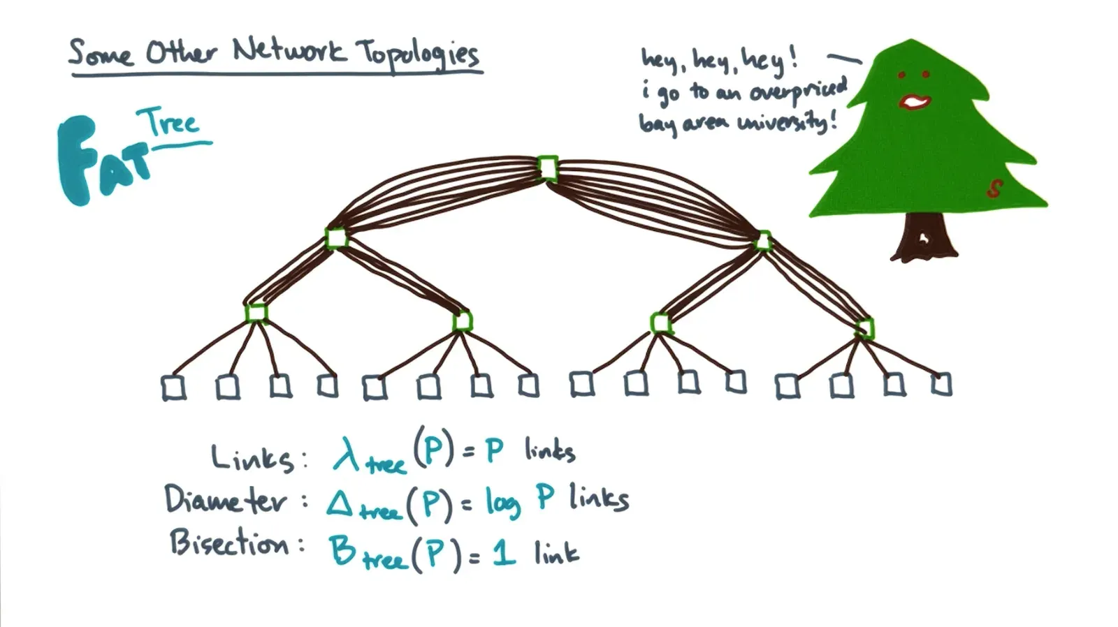
- Make fat tree by adding more links the higher level you go
- Toruses have more links but reduce the diameter and bisection and are used in many supercomputers
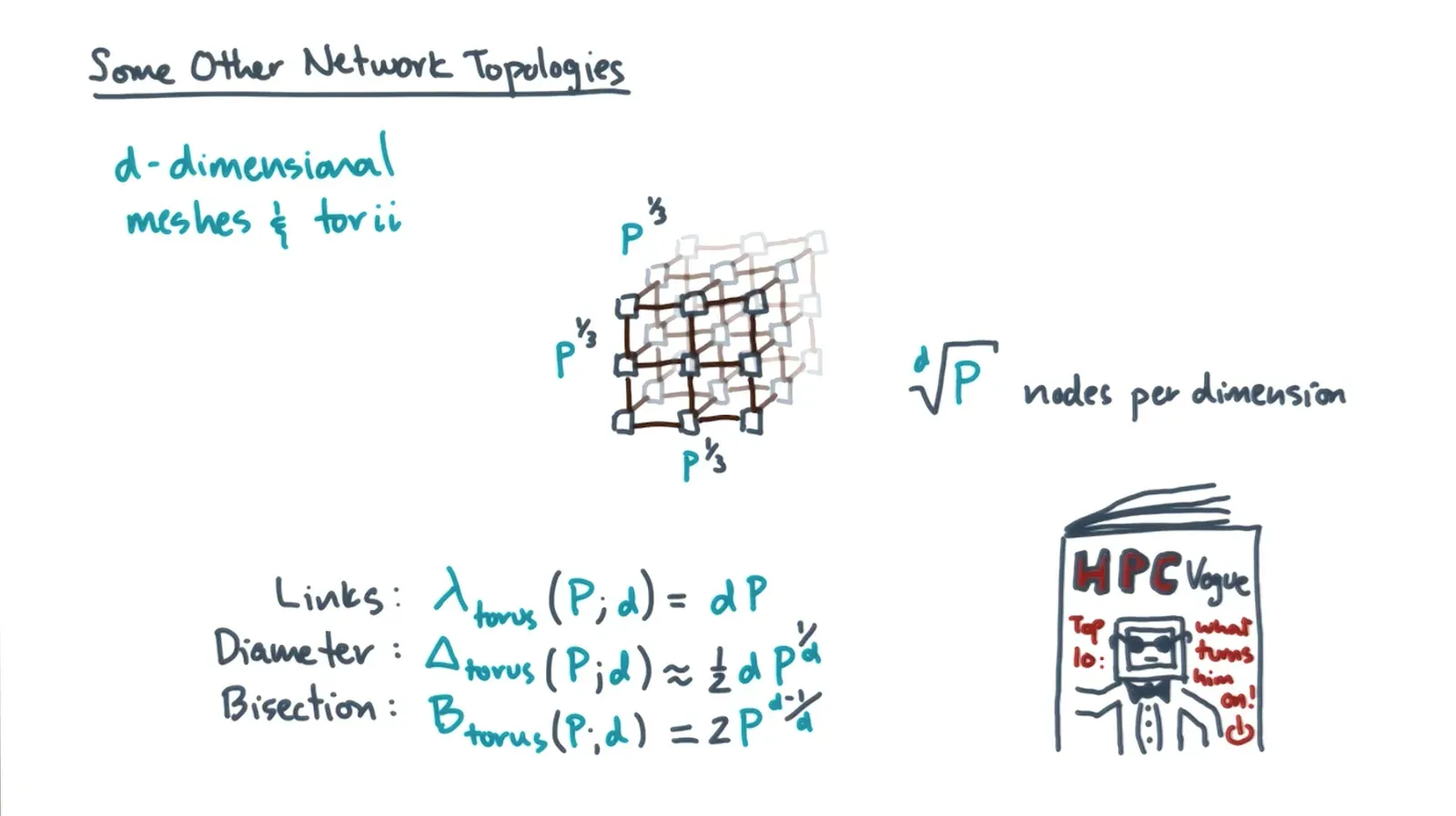
- Hypercubes not used in application but talked a lot about in theory
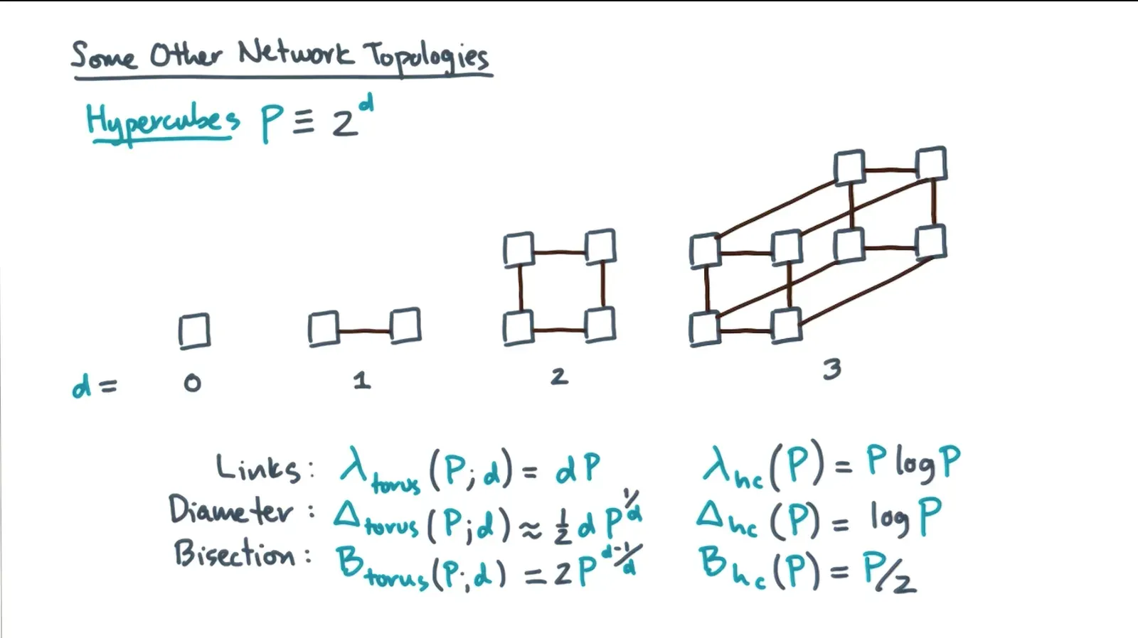
- Trees have scalable links and diameter but poor bisection as only 1 way to transfer
- Changing network models can either introduce or remove congestion which is the number of logical edges that map to physical ones
- Can estimate congestion increase/decrease by dividing Bisection widths of logical/physical
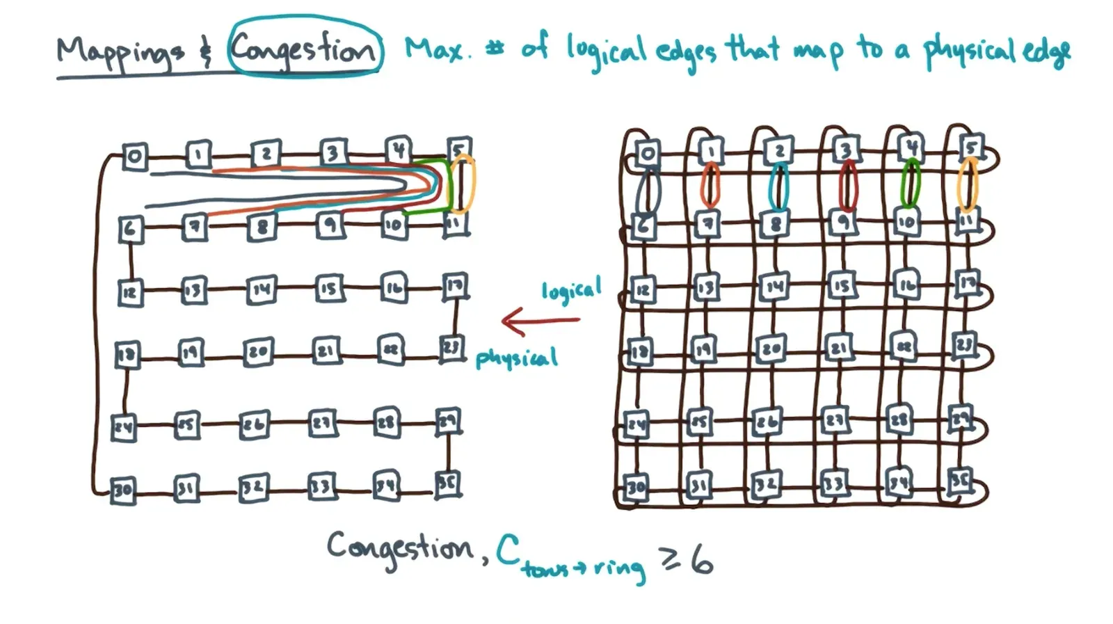
- Can estimate congestion increase/decrease by dividing Bisection widths of logical/physical
- On higher dimension meshes, it takes less time to do all to all operations if model allows
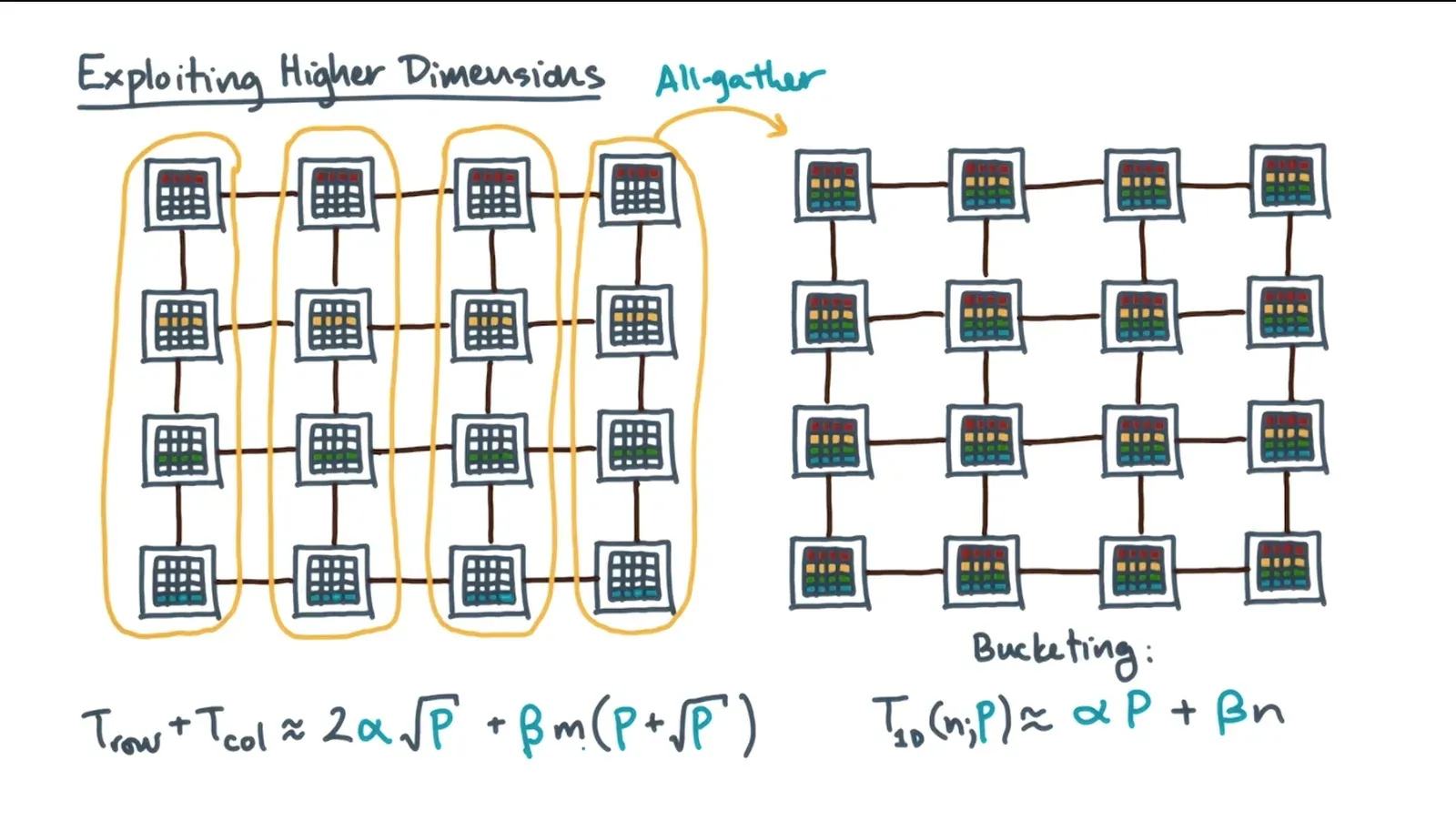
- All to All collective nodes want to send a unique message to all other nodes
- For every iteration, ship off all data that isnt needed per node to the next node in a circular fashion
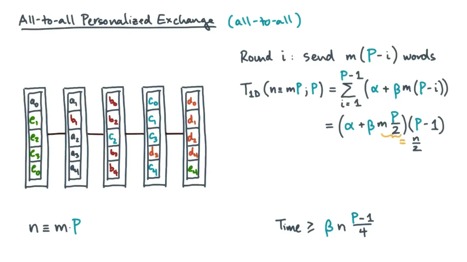
- For every iteration, ship off all data that isnt needed per node to the next node in a circular fashion
Distributed Dense Matrix Multiply
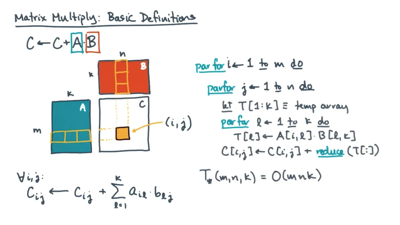
- Can paralellize matrix multiply with work O(n^3) and span O(log(n))
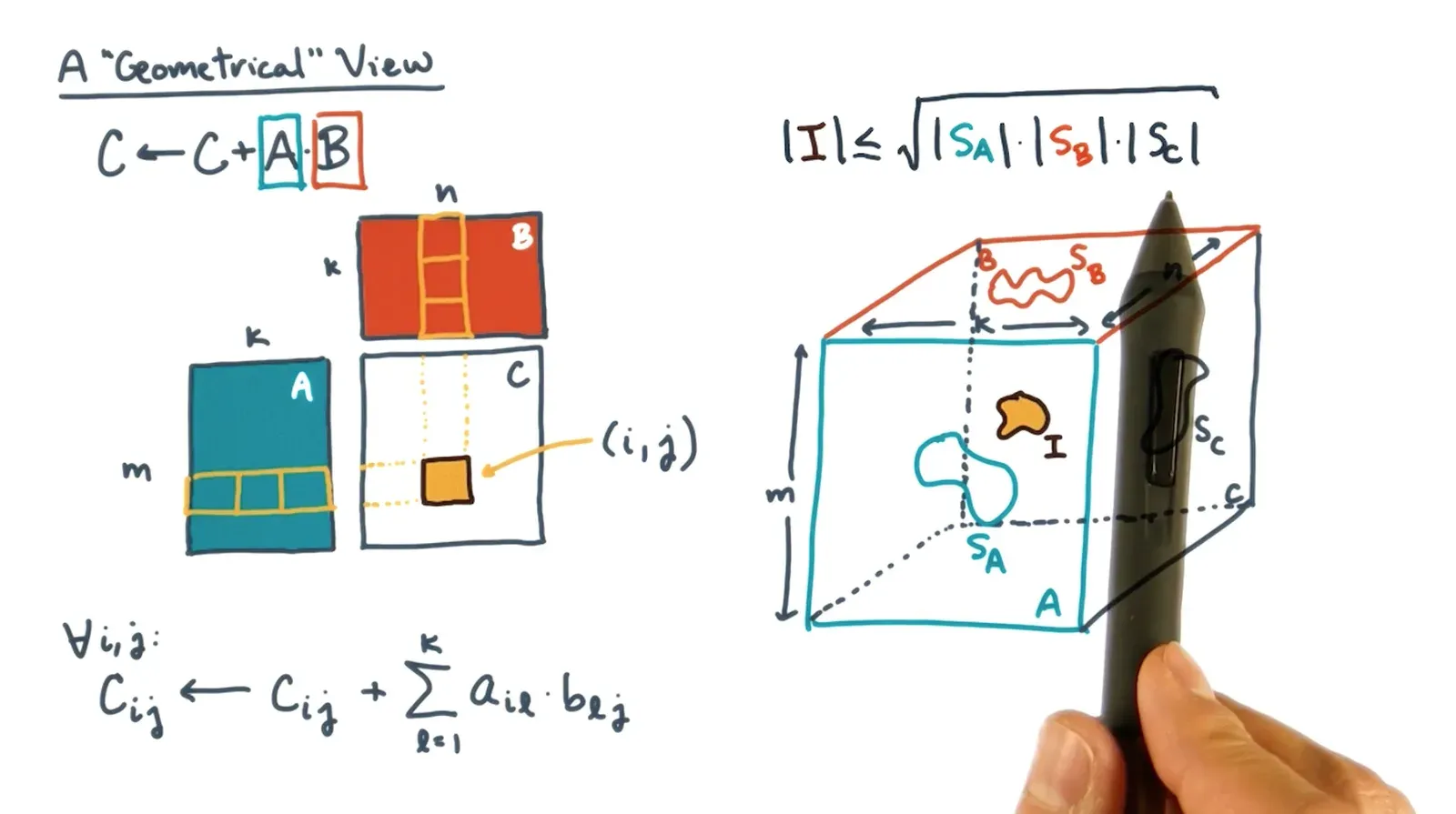
- Visualize parallel matrix multiply as a cube where the volume of I (an area) is at most the square root product of areas SA SB and SC (Loomis Whitney Theorem)
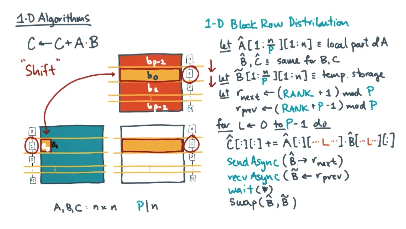
- Distributed matrix multiply with MPI involves shifting rows around while doing the multiply every block(s)
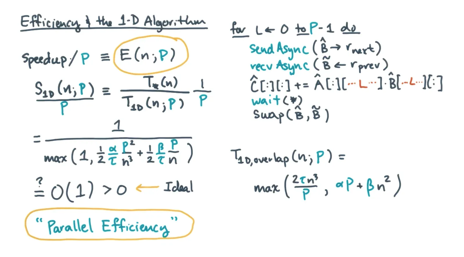
- Speedup / P OR Sequential Time / Parallel Time * P is parallel efficiency and aim to keep it at a constant
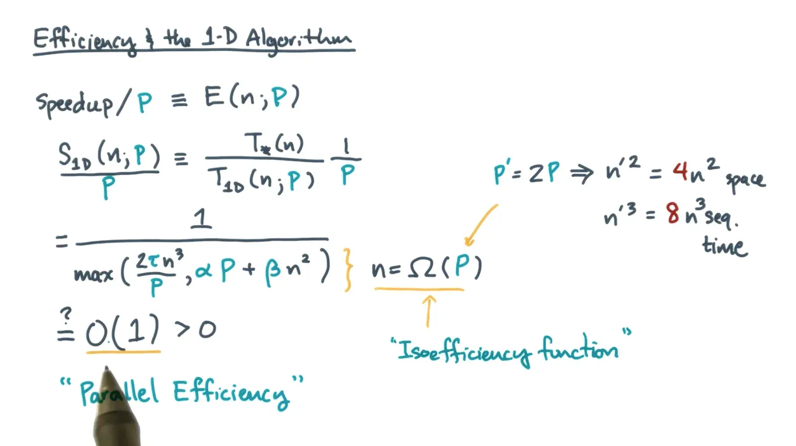
- IsoEfficiency function function of P that n must satisfy in order to have constant parallel efficiency
- SUMMA 2D Matrix Algorithm loops accross strips of both matrices and every strip is broadcasted to other rows/columns for usage
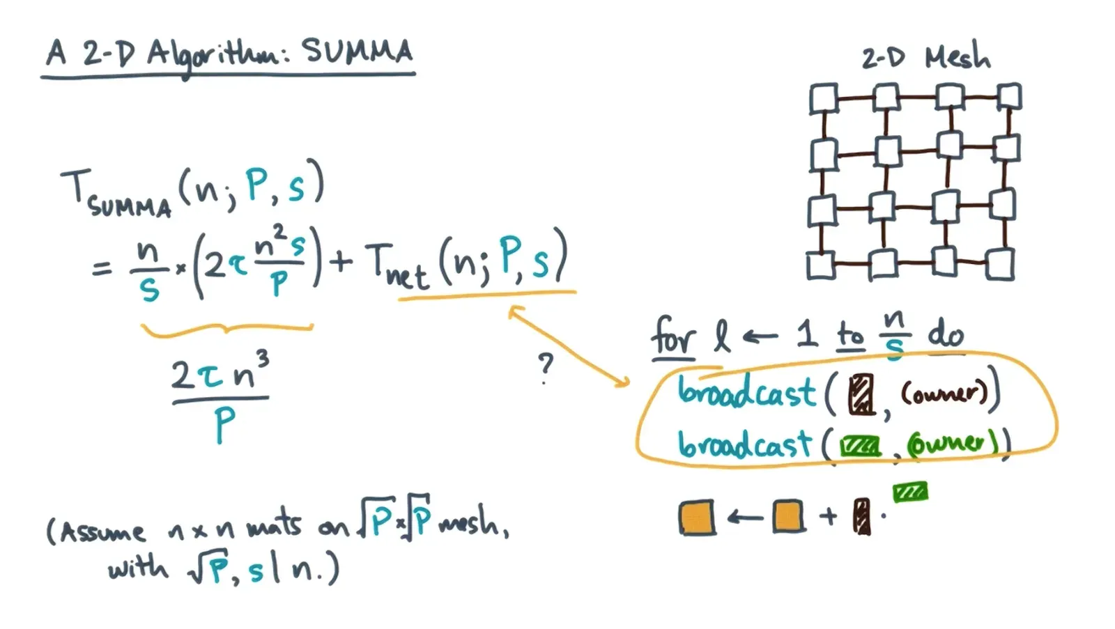
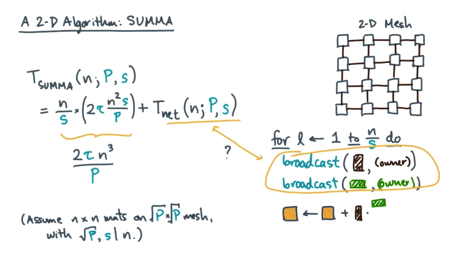
- More optimal than 1D
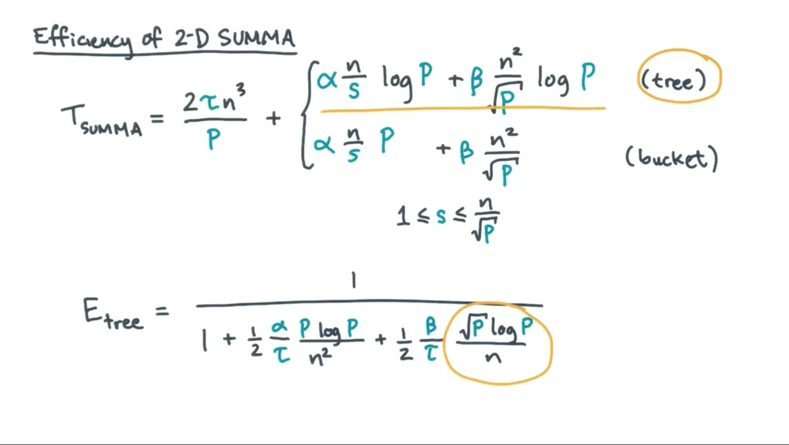
- More optimal than 1D
- Lower bound analysis of SUMMA 2D Algorithm
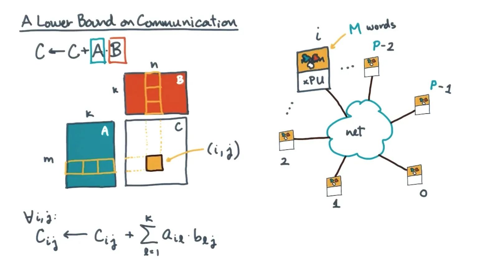
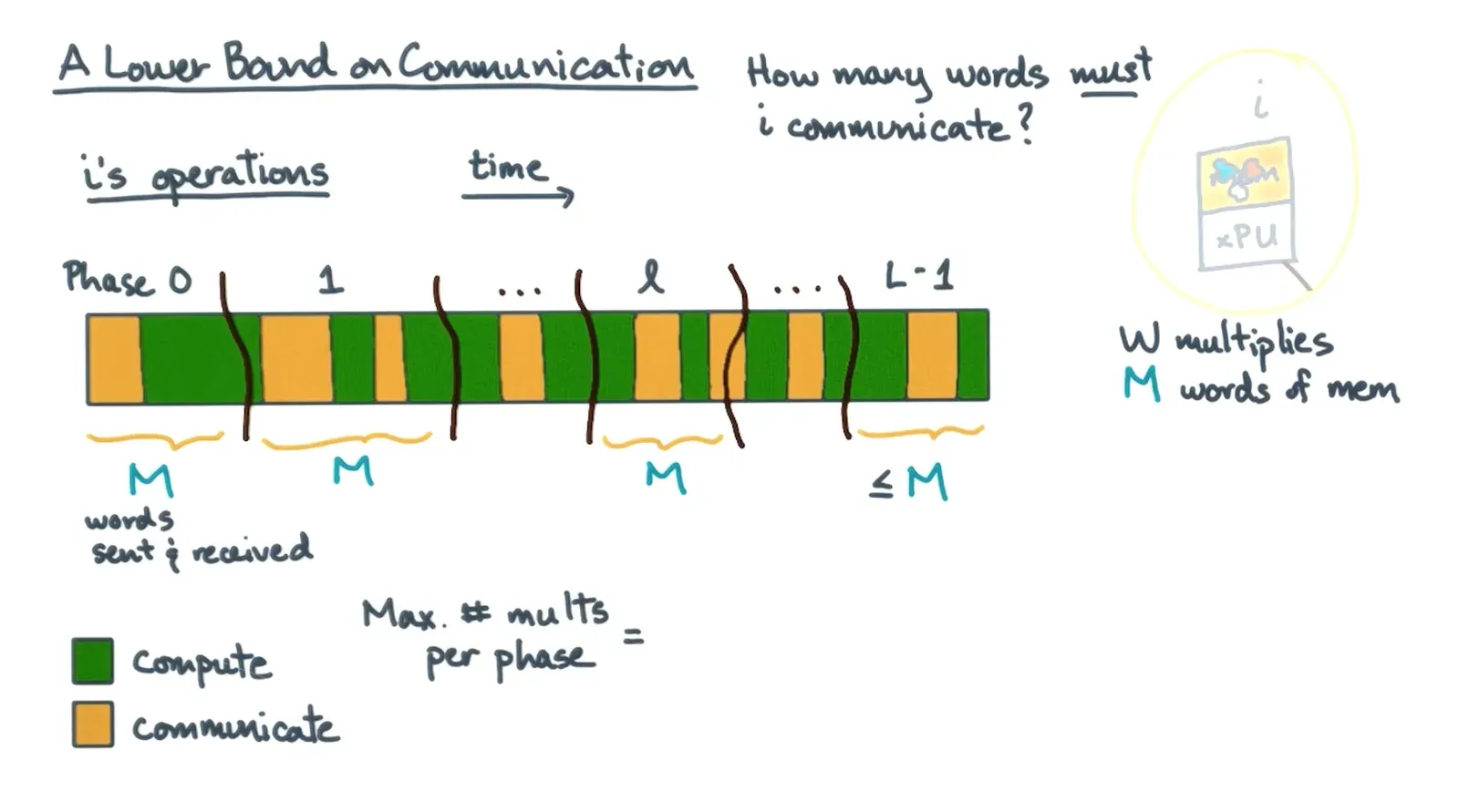
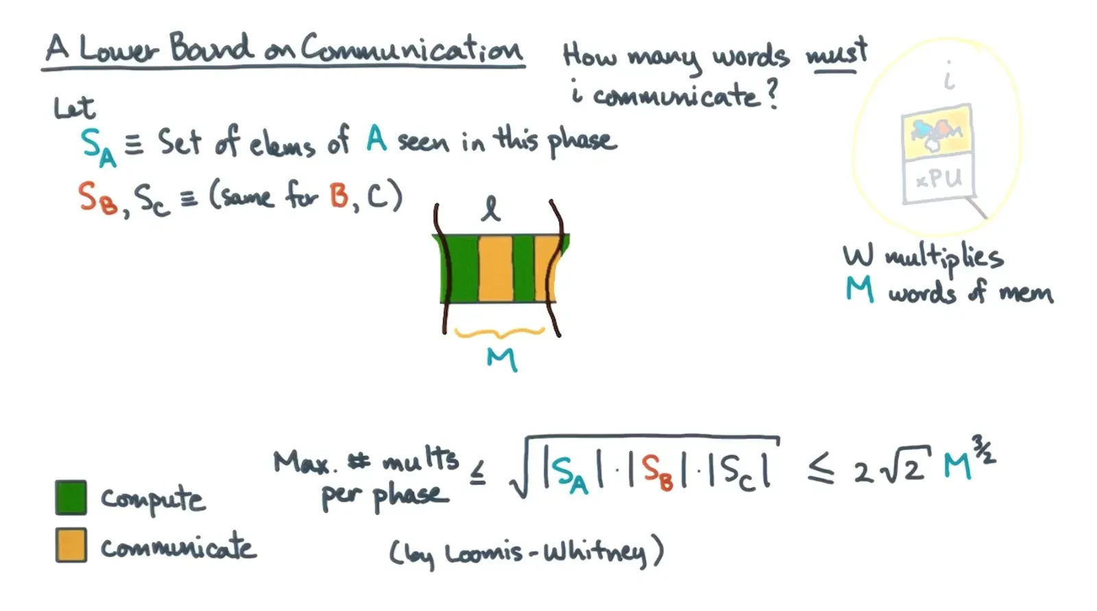
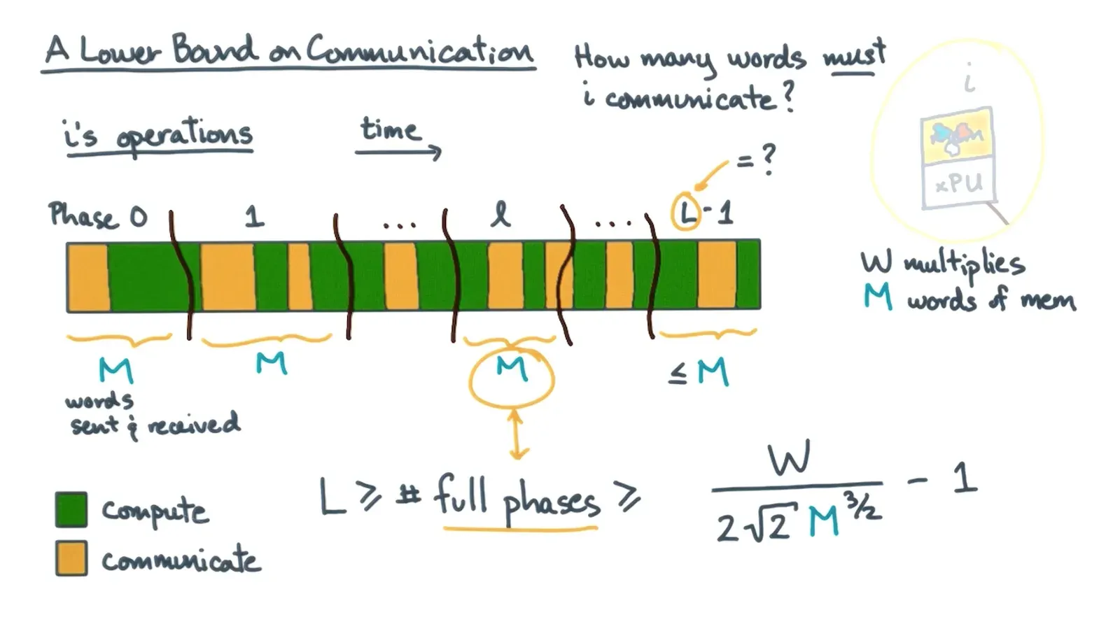
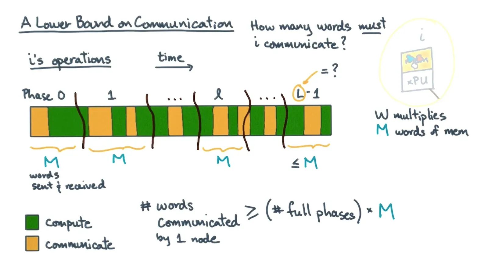
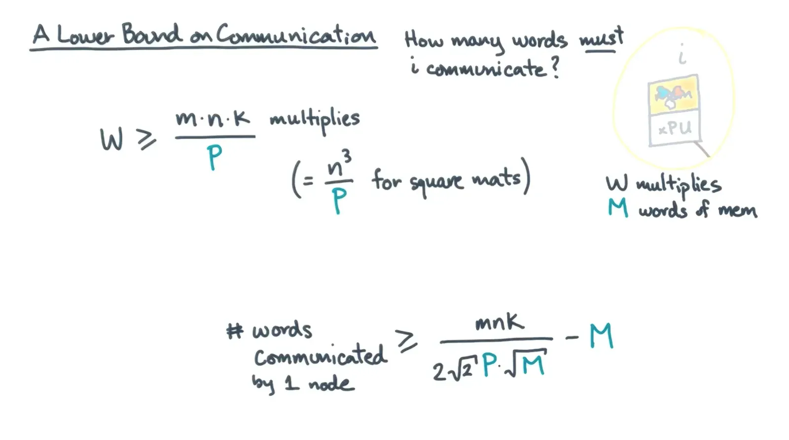
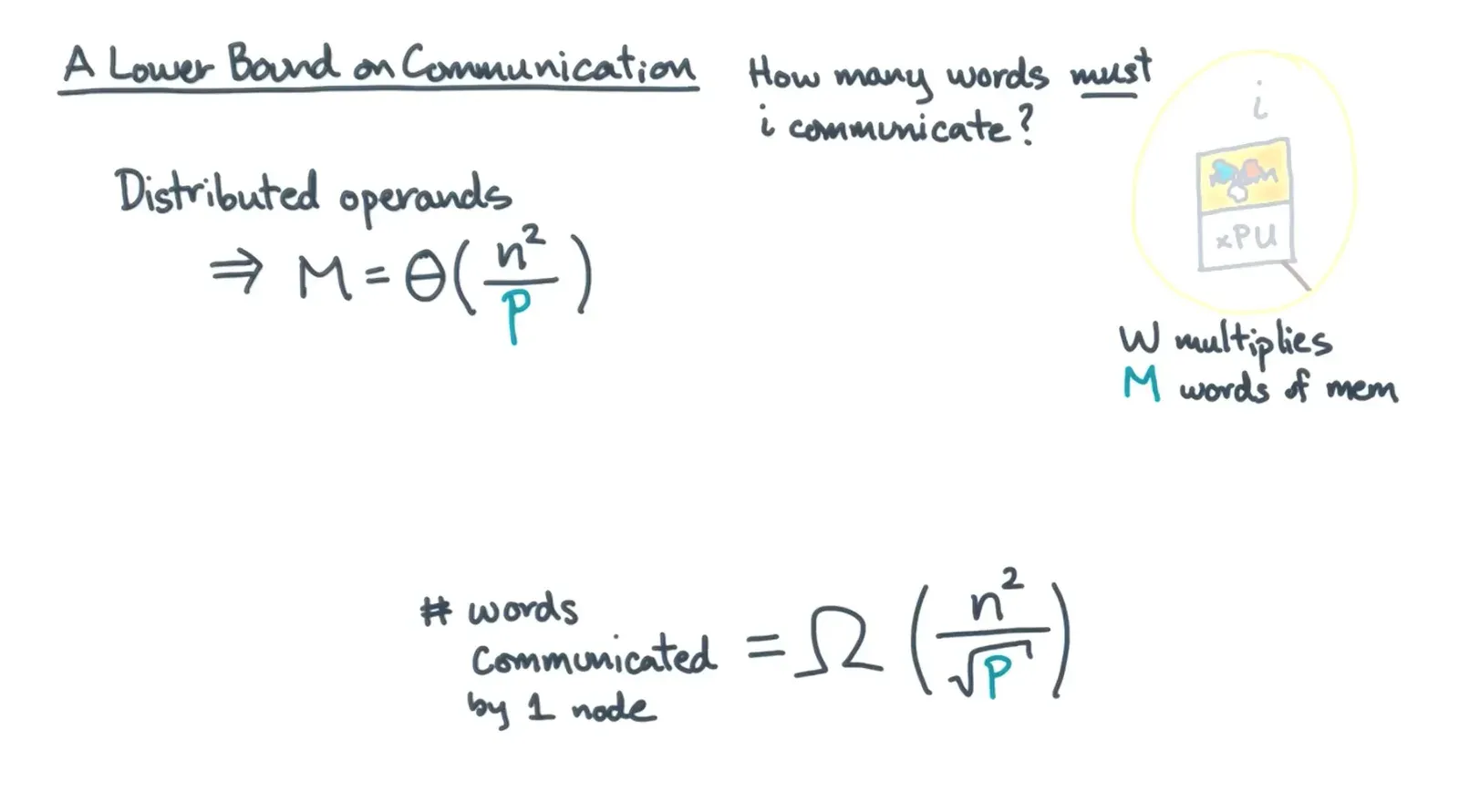
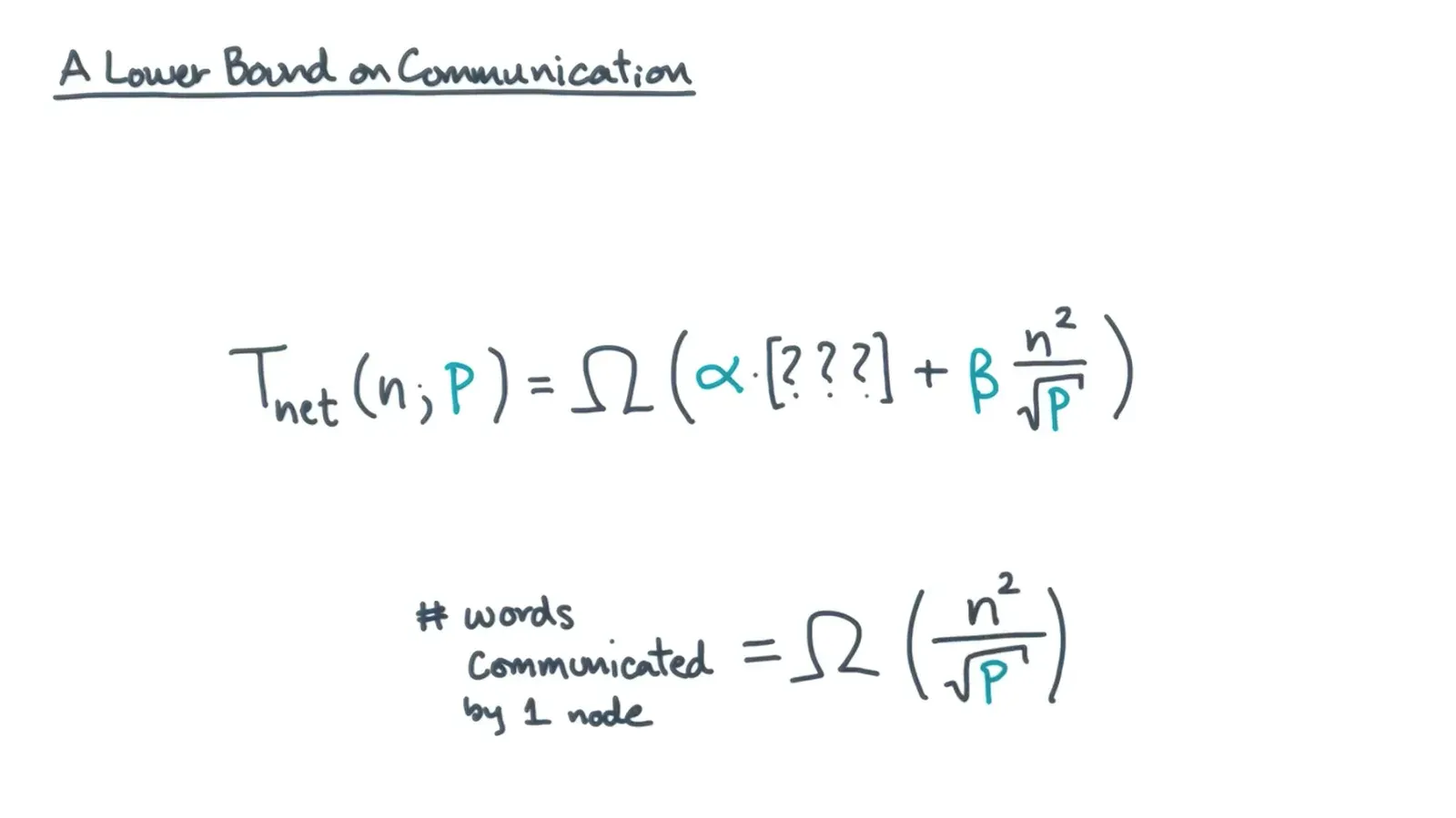
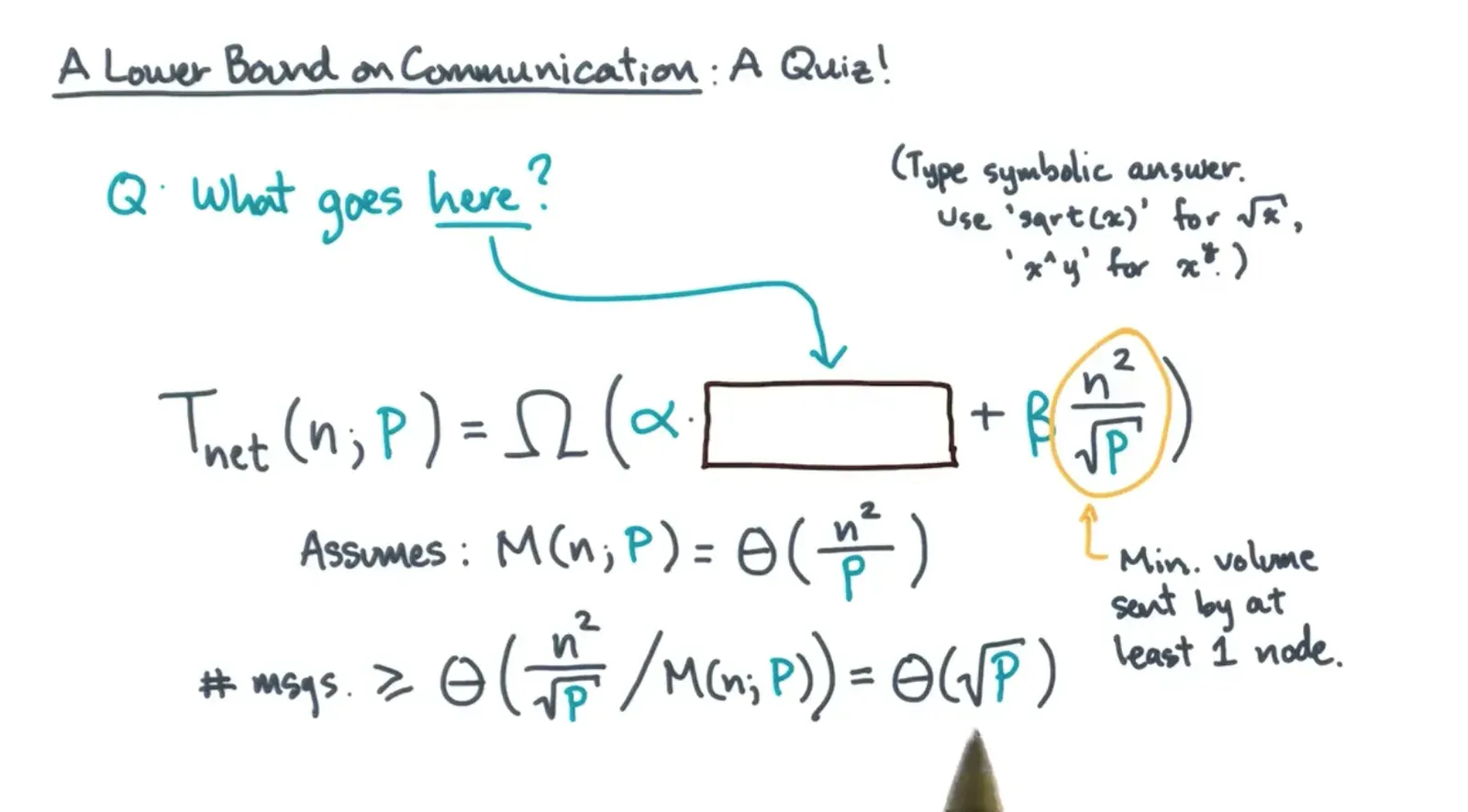
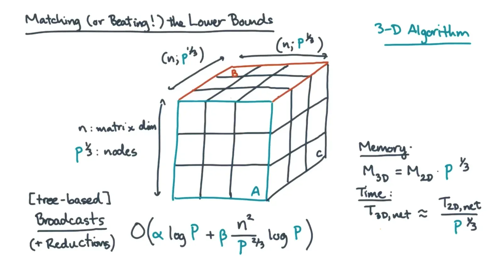
- Can beat the lower bound by using a 3D mesh or Cannon’s Algorithm which reduces the communication requirement but increases the amount of memory used
Distributed Memory Sorting
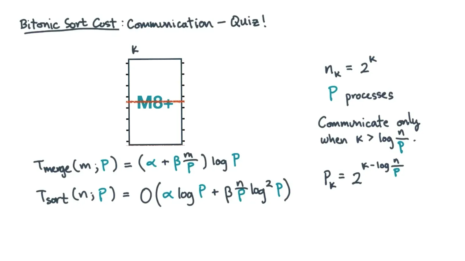
- For distributed bitonic merge w/ binary exchange can divide up the elements among nodes
- Will be log P communication steps for exchanging data for bitonic split and log n/P local steps for bitonic merge itself
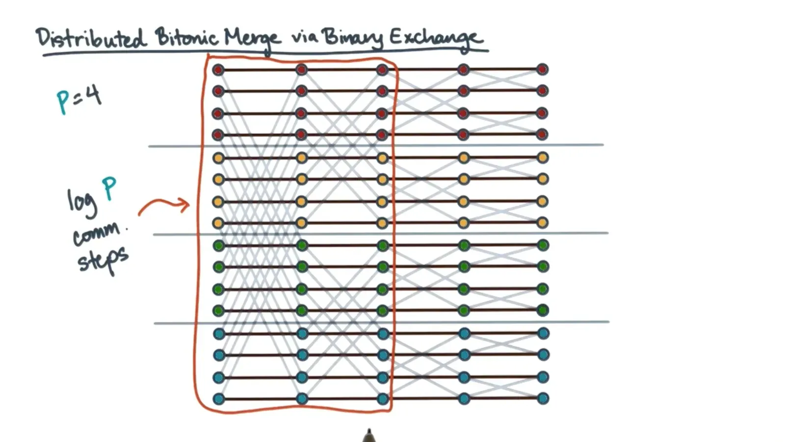
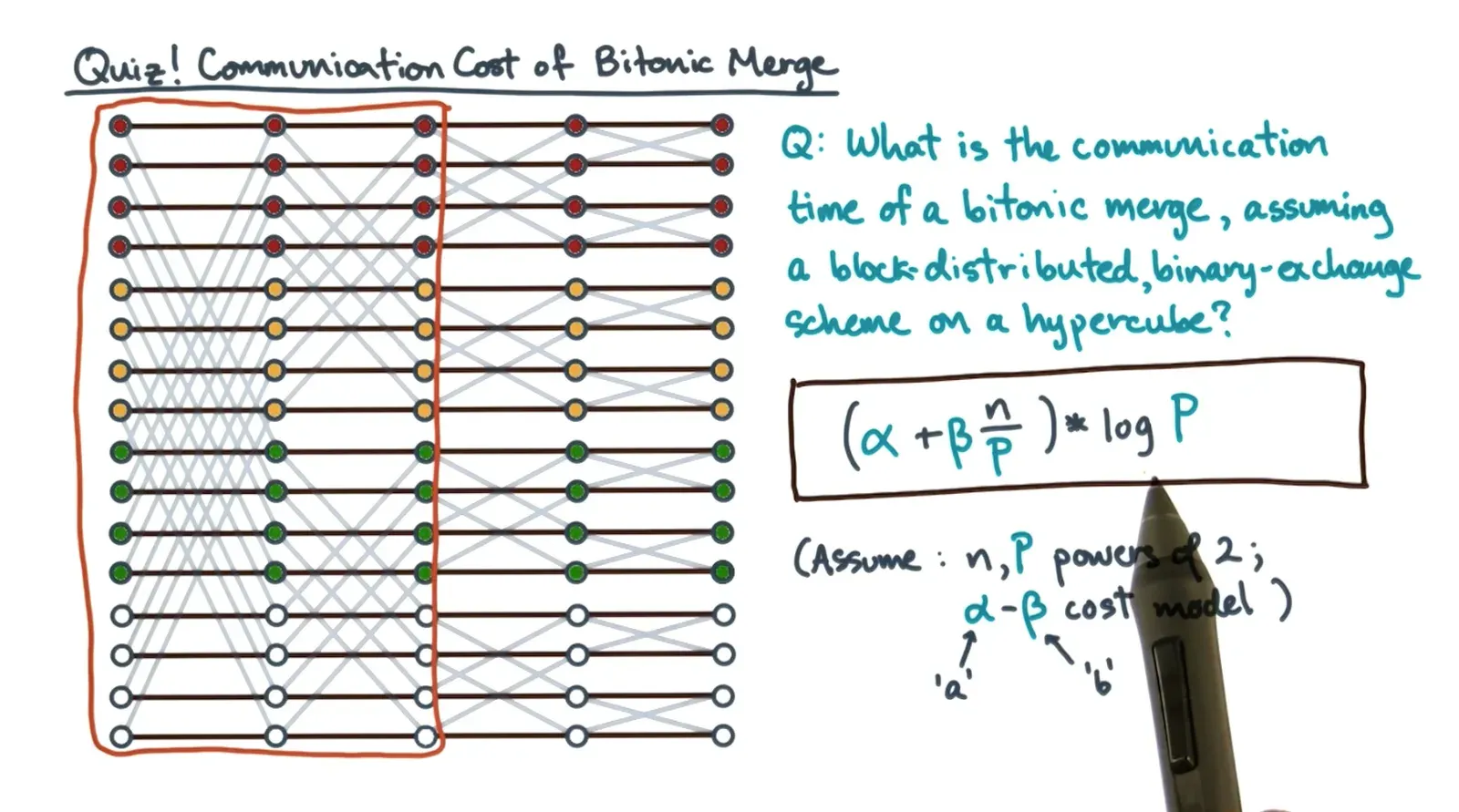
- Will be log P communication steps for exchanging data for bitonic split and log n/P local steps for bitonic merge itself
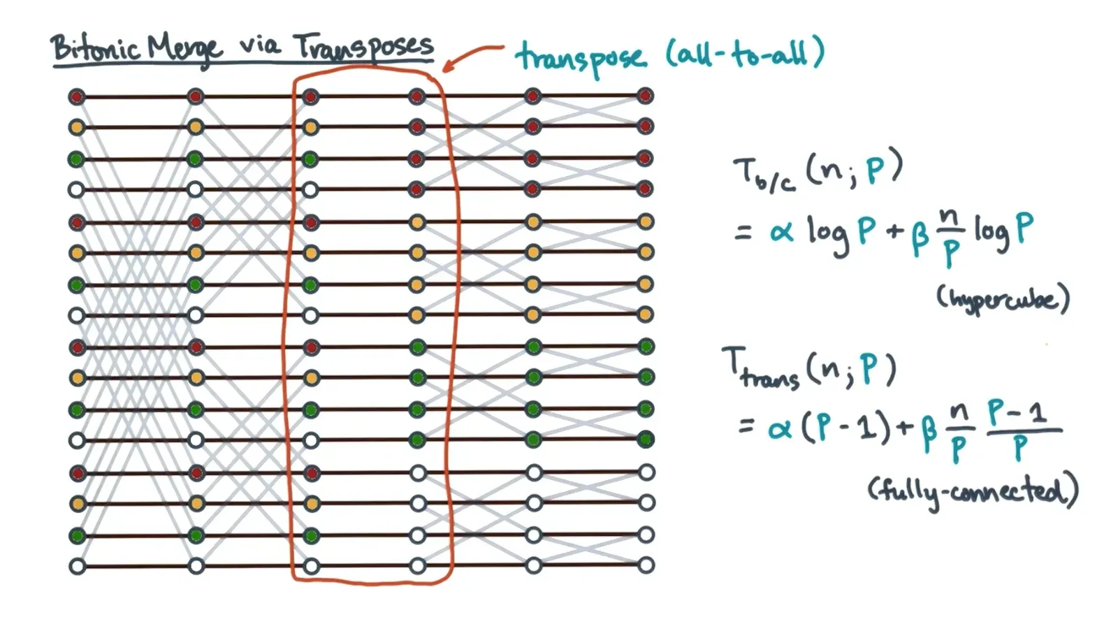
- Can do bitonic merge with transposes where you reduce the cost of datasend(beta) but increase cost of message preparation(alpha)
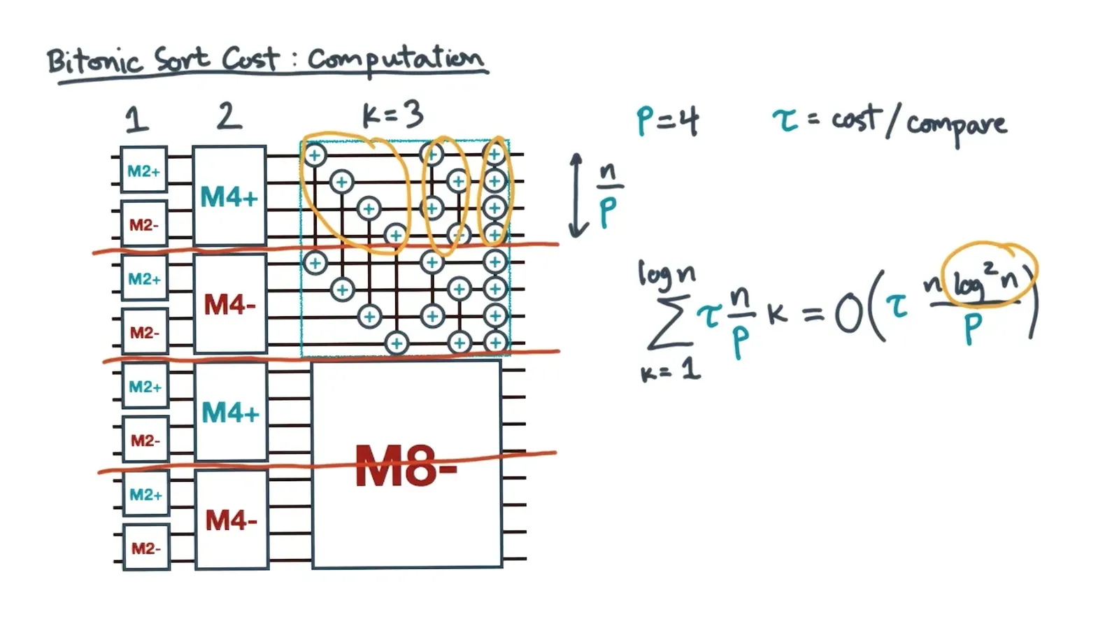
- Computation and communication cost of bitonic sort:
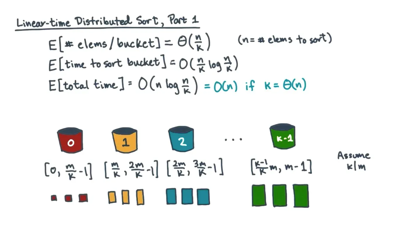
- Can implement a distributed bucket sort by grouping elements in buckets, sorting the elements within each bucket, and then combining them together but must choose a k properly
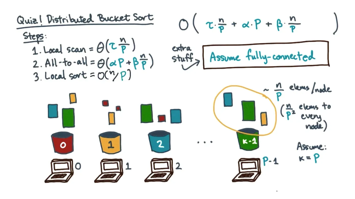
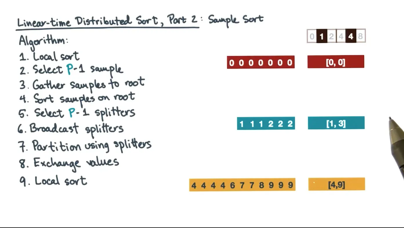
- Can use sampling to make buckets more balanced and then perform sort that way
Distributed BFS
- First store graph as an adjacency matrix
- Then for frontier nodes in an array and the array, do a matrix vector multiply such that we have the nodes to update next iteration
- Then with update array, update distances and frontier array
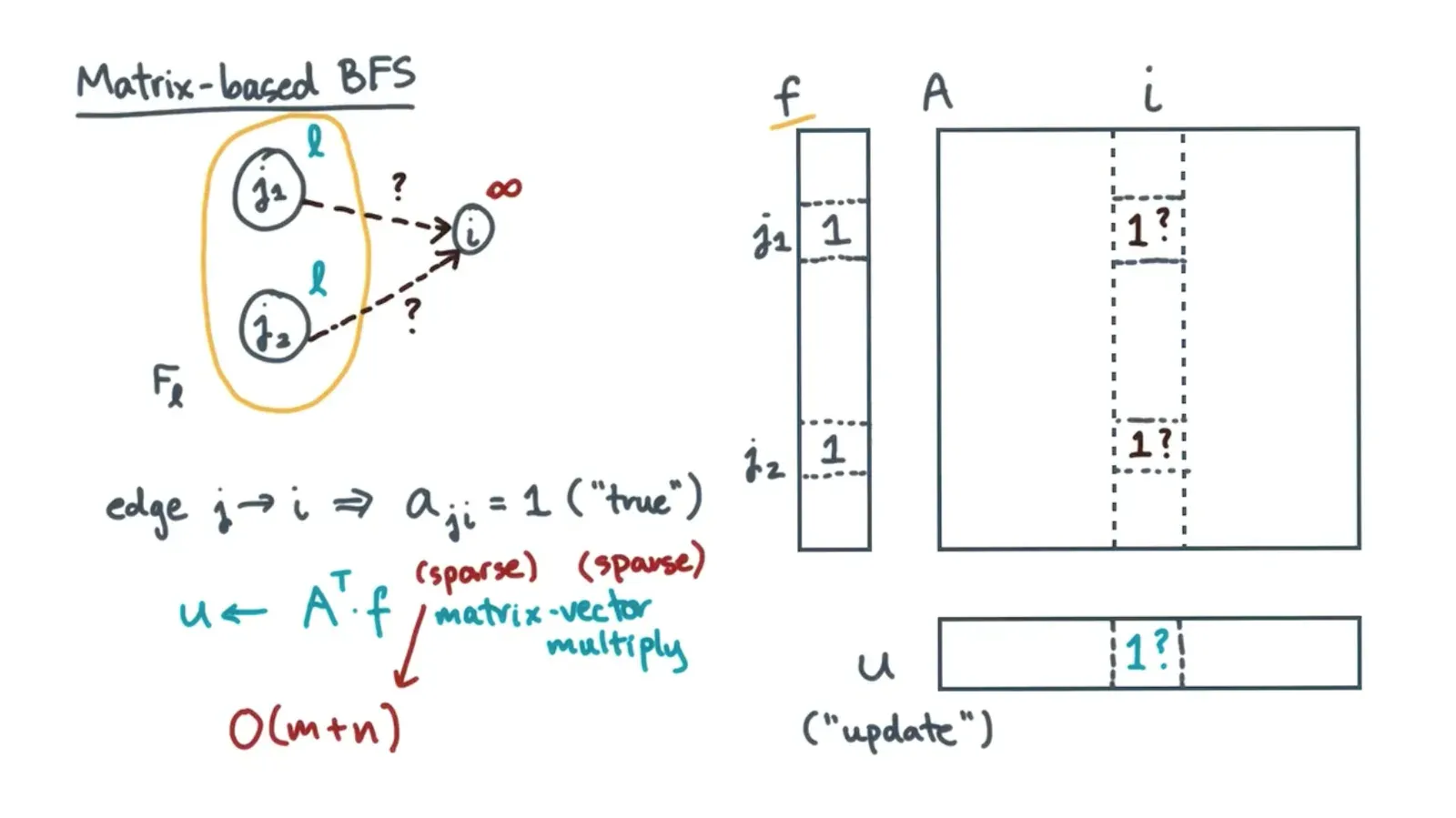
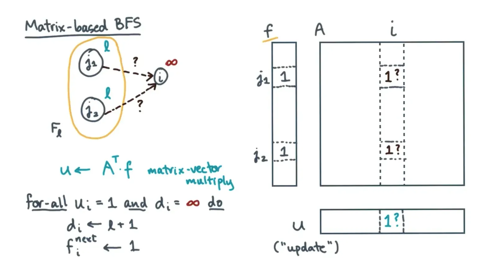
- Then with update array, update distances and frontier array
- To distribute the BFS, partition the adjacency matrix per process and replicate the frontier array on every process
- Then when updating the new frontier array, need to do an all to all exchange
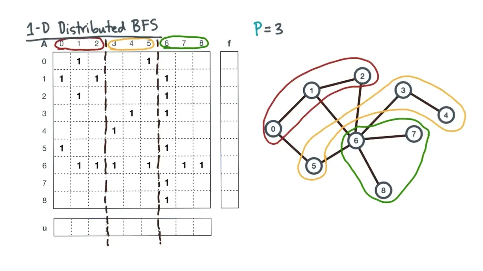
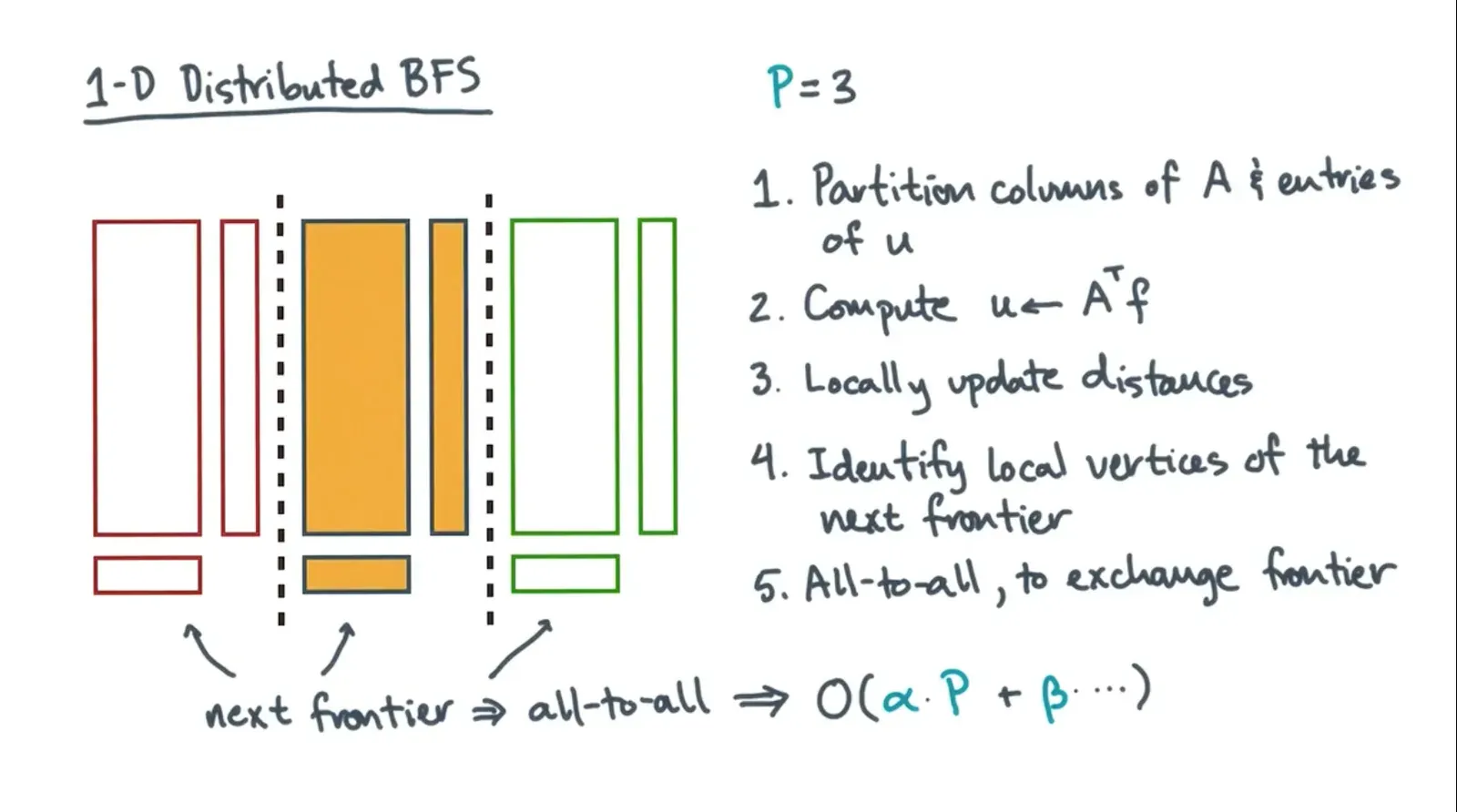
- Then when updating the new frontier array, need to do an all to all exchange
Graph Partitioning
- In distributed BFS we need to choose partitions carefully in order to balance work (based on number of non zeroes) and minimize edge cuts
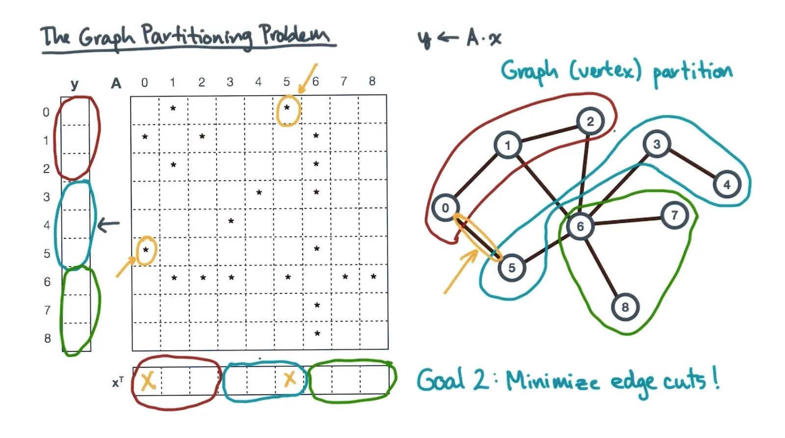
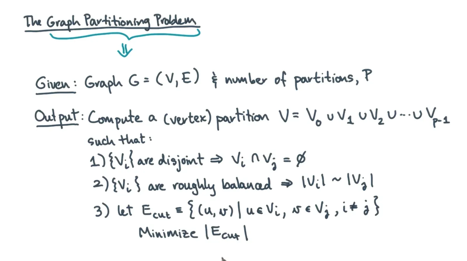
- Graph partitioning problem states that we should find a vertex partition such that all sets are disjoint, roughly balanced, and minimize edge cuts
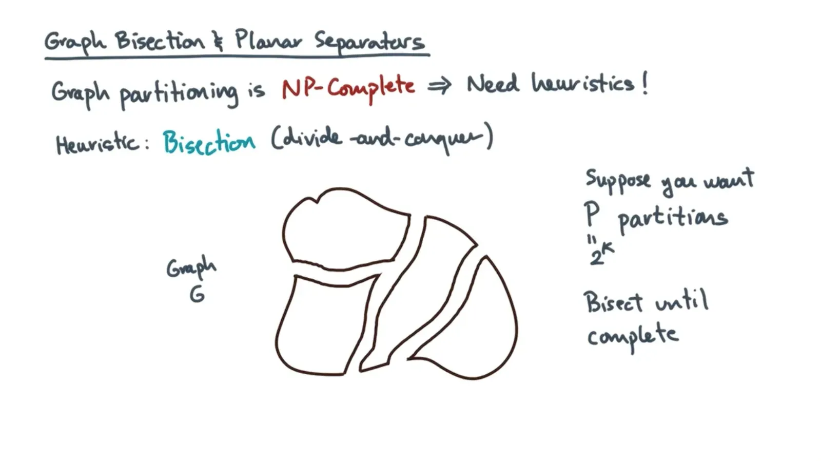
- Graph partitionings can be done with bisections splitting into 2 - how to do this in theory?
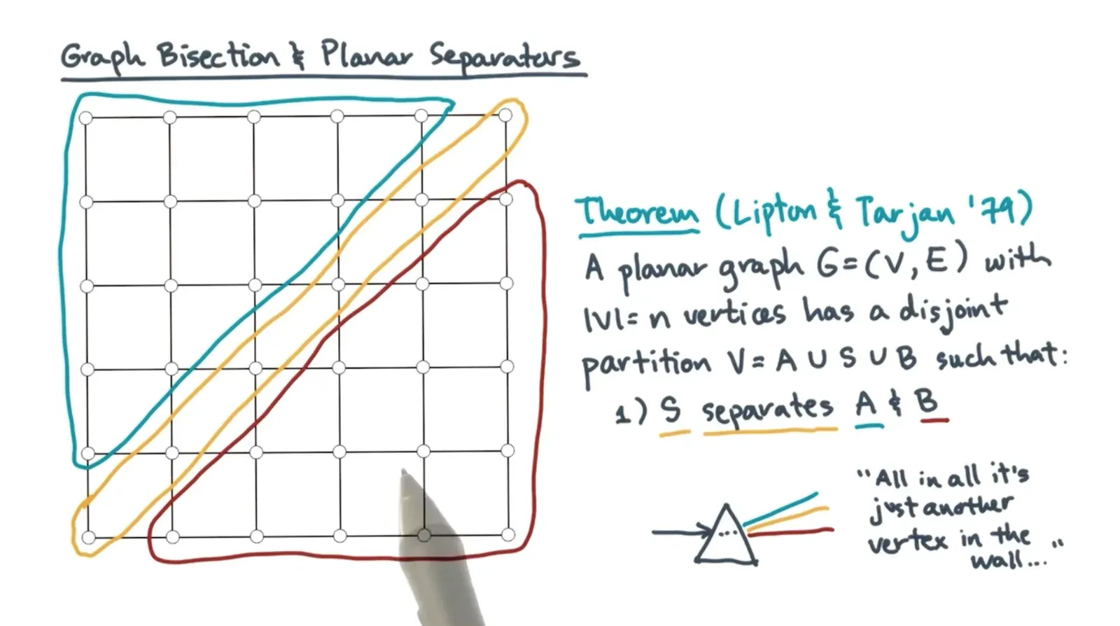
- Use planar graphs where
- The separator partition S separates sets A and B
- Size of A and B are ≤ 2/3n so A and B differ less than factor of 2 (balanced)
- Size of S is ~sqrt(n)
- Use planar graphs where
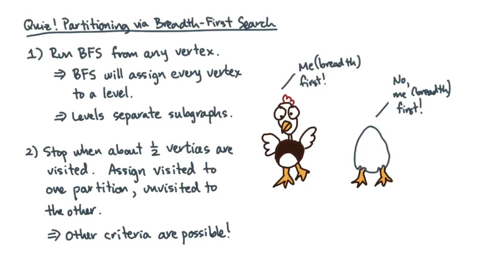
- Can create a graph partitioning via BFS
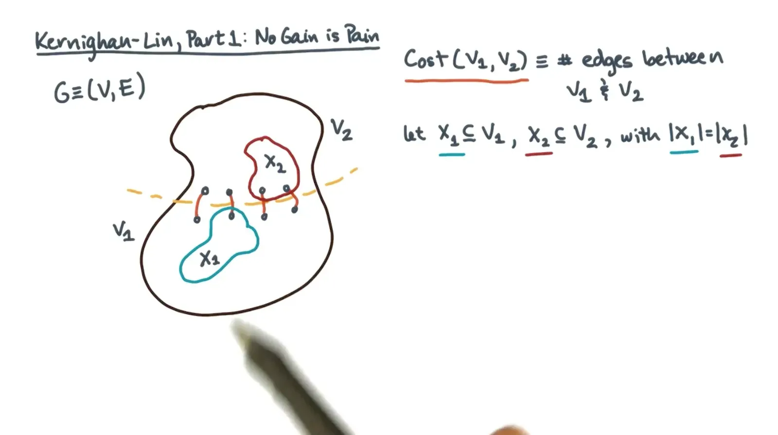
- Kernighan Lin involves partitioning the graph with any partition but how to figure out the cost?
- Take external cost edges of a going to V2 + external cost edges of b going to V1 - any possible extraneous edge + Cost(V1 - a, V2 - b)
- If you swap a and b then invert the above with internal cost edges
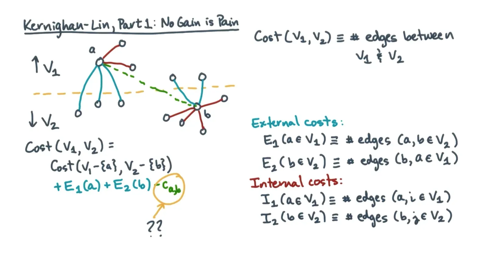
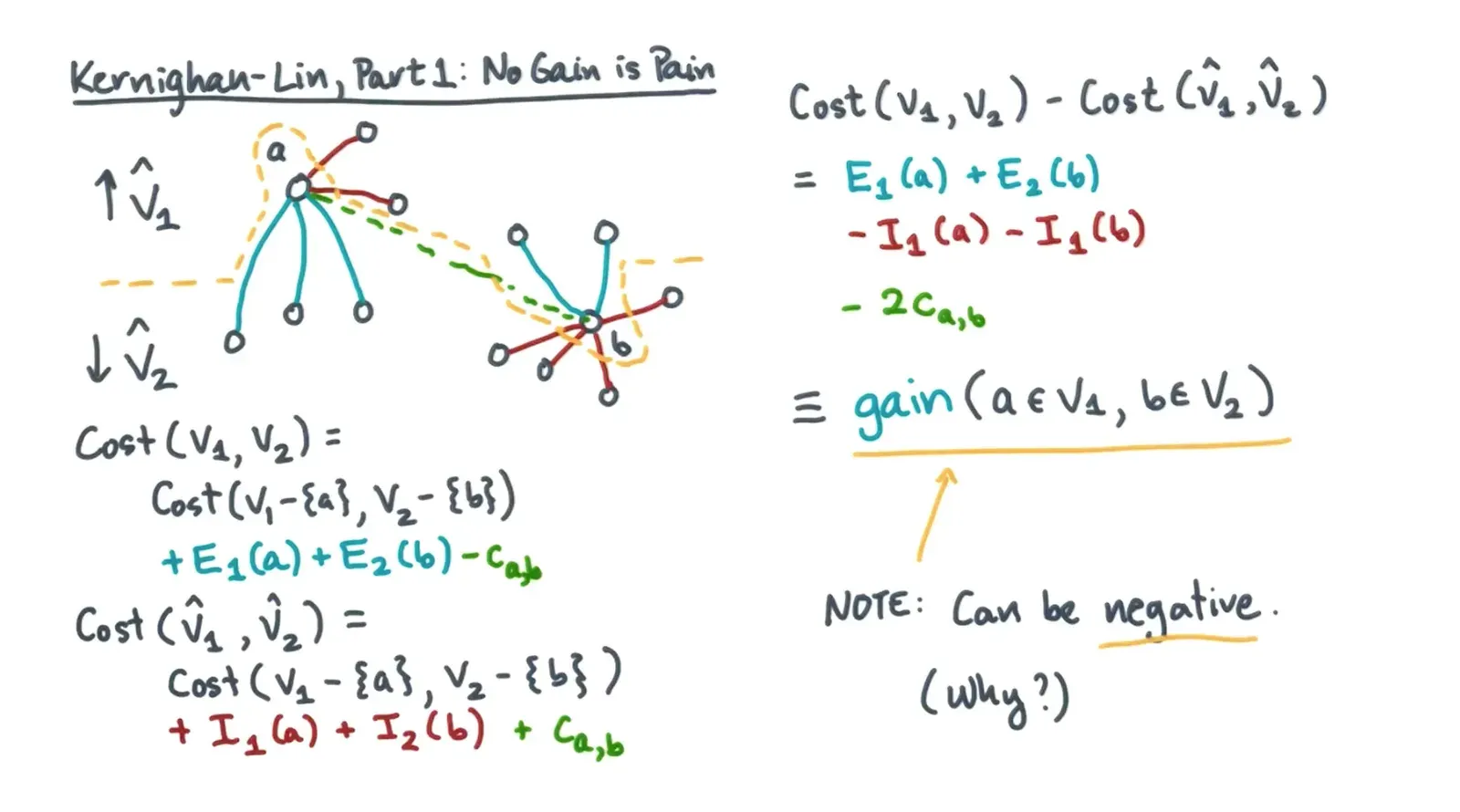
- Kernighan Lin Algorithm has multiple parts with time complexity of O(V^2 * d)
- First compute the sequence of gains for (a1, b2), (a2, b2)…
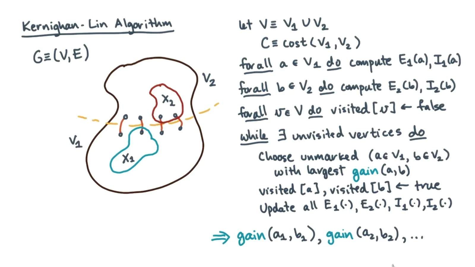
- Then keep trying to compute cumulative gains and record cost - gain every iteration until cumulative gain is less than 0
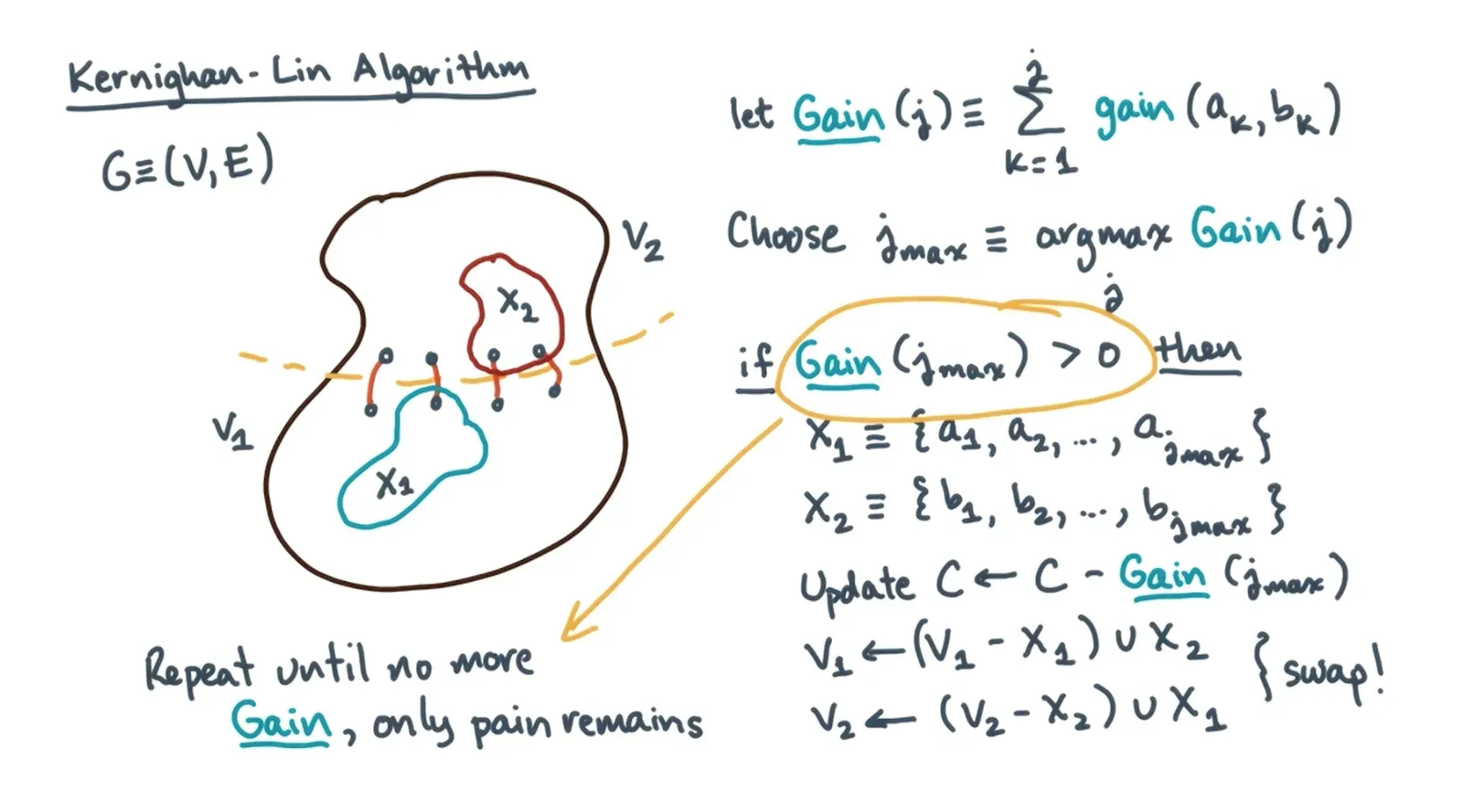
- First compute the sequence of gains for (a1, b2), (a2, b2)…
- Graph coarsening involves shrinking the graph just enough such that it preserves all necessary information but looks like the original graph
- Need to update vertices to weights map along with edges to weights map if we merge vertices/edges together into a super node
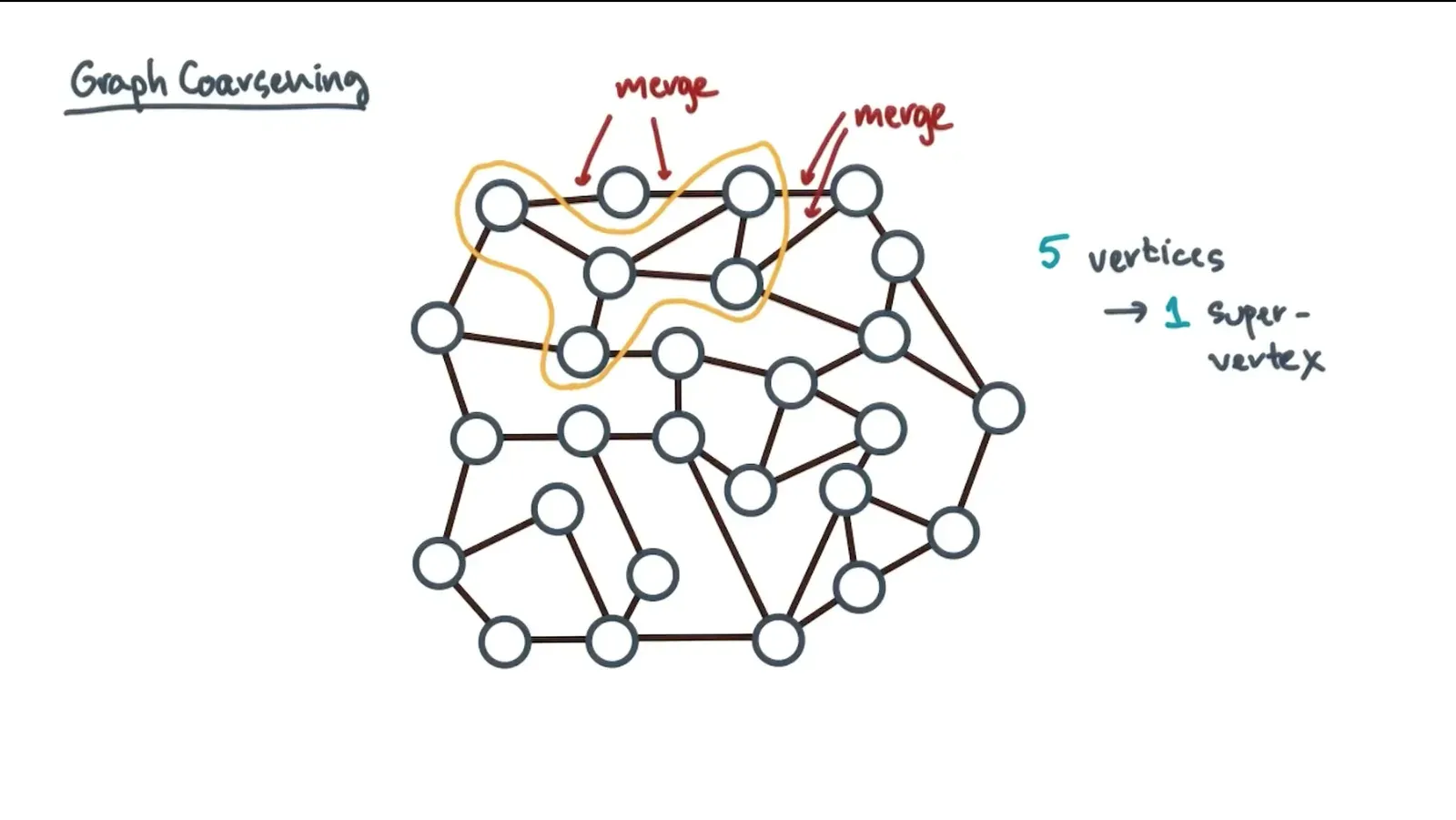
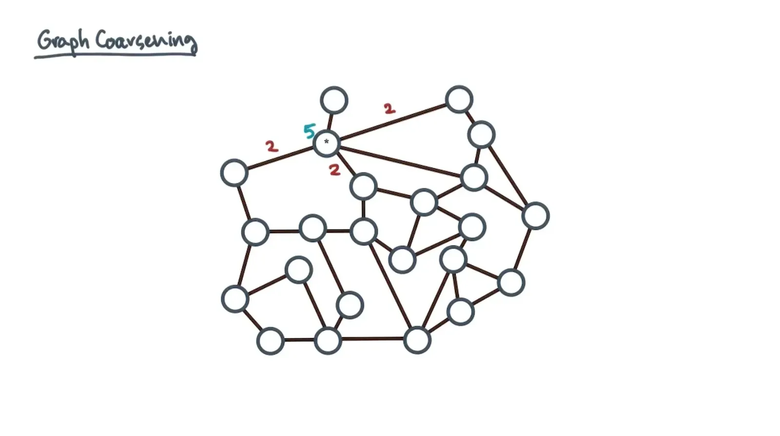
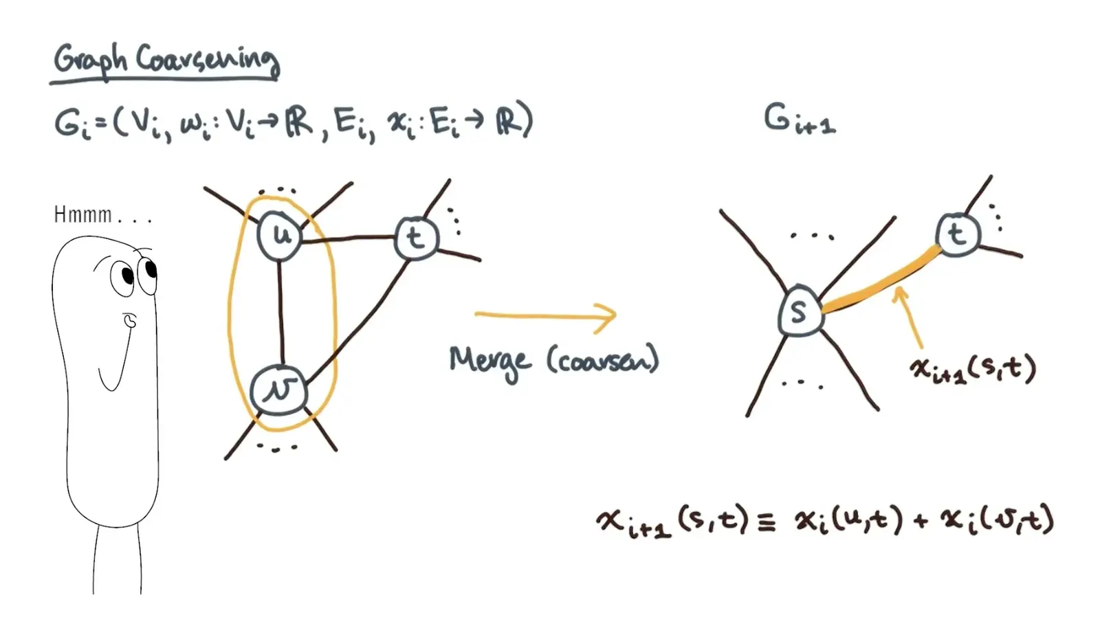
- Need to update vertices to weights map along with edges to weights map if we merge vertices/edges together into a super node
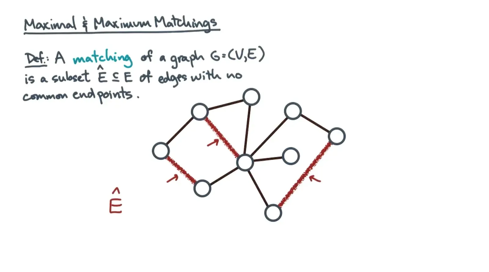
- You need a scheme to figure out which vertices to combine in graph coarsening ⇒ maximal/maximum matchings
- Matching of a graph is set of vertices where all of them share no common endpoints
- Maximal matching is matching where you can’t add any more edges
- Maximum matching is matching with the most amount of edges one could add
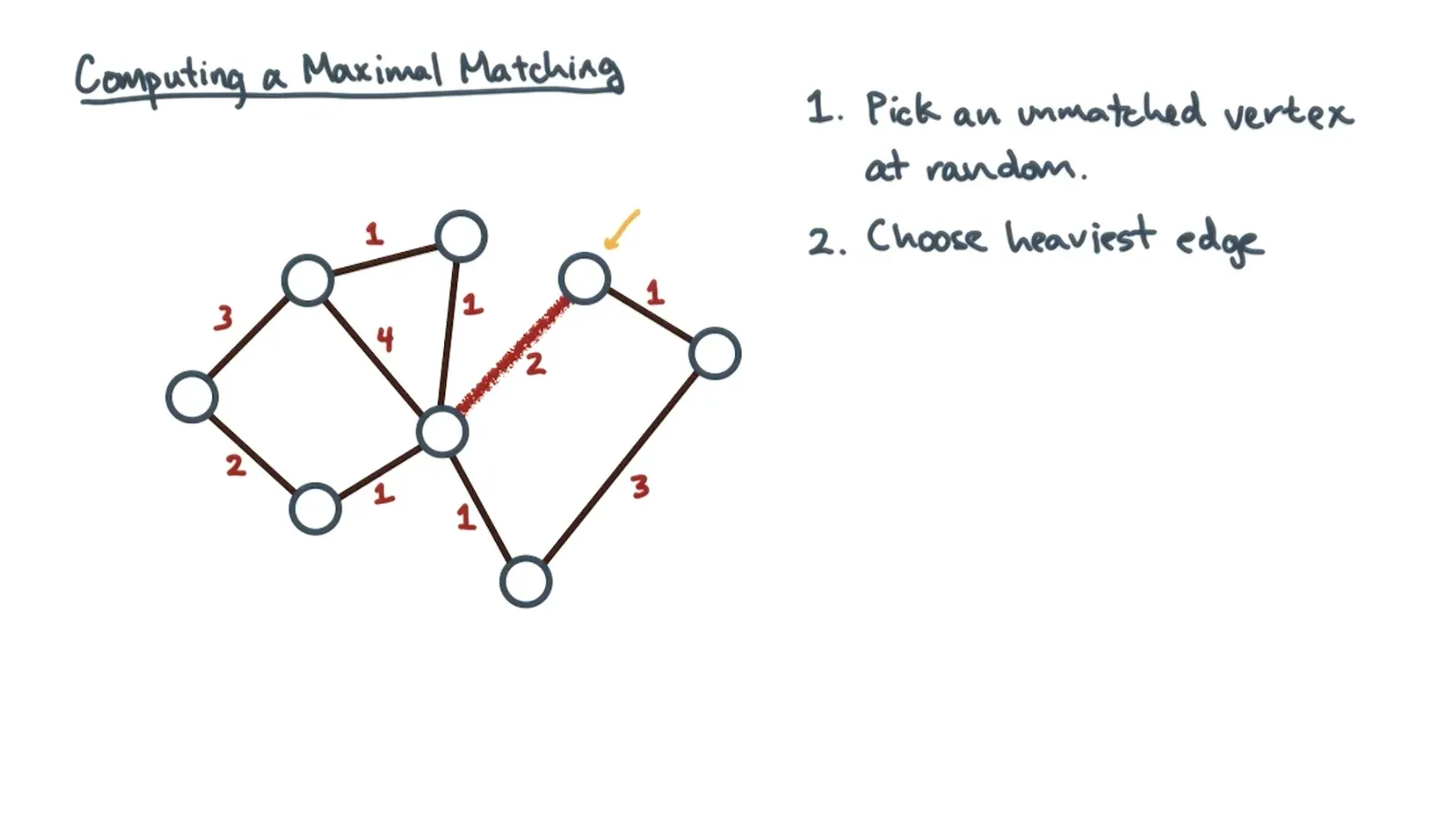
- Computing maximal matching involves picking an unmatched vertex at random and choosing the heaviest neighboring edge to match on
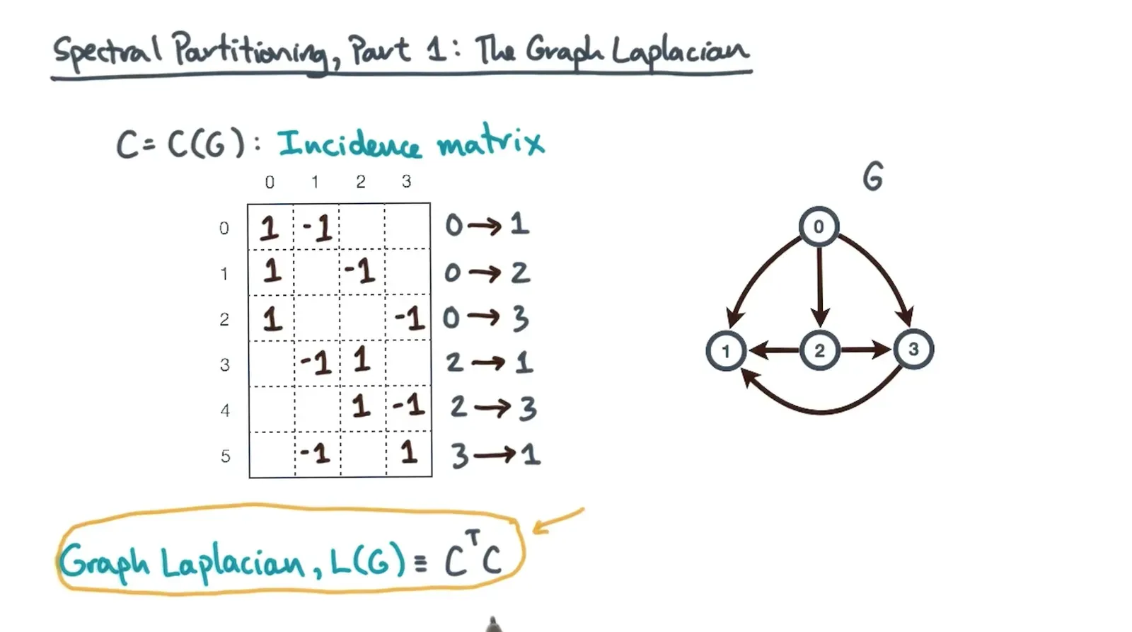
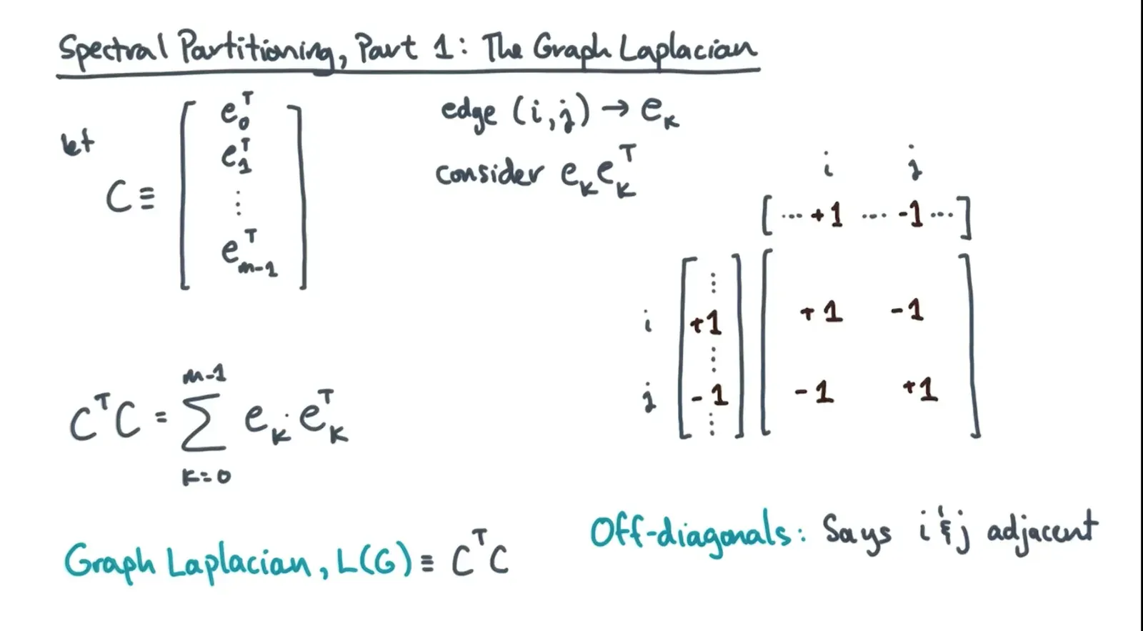
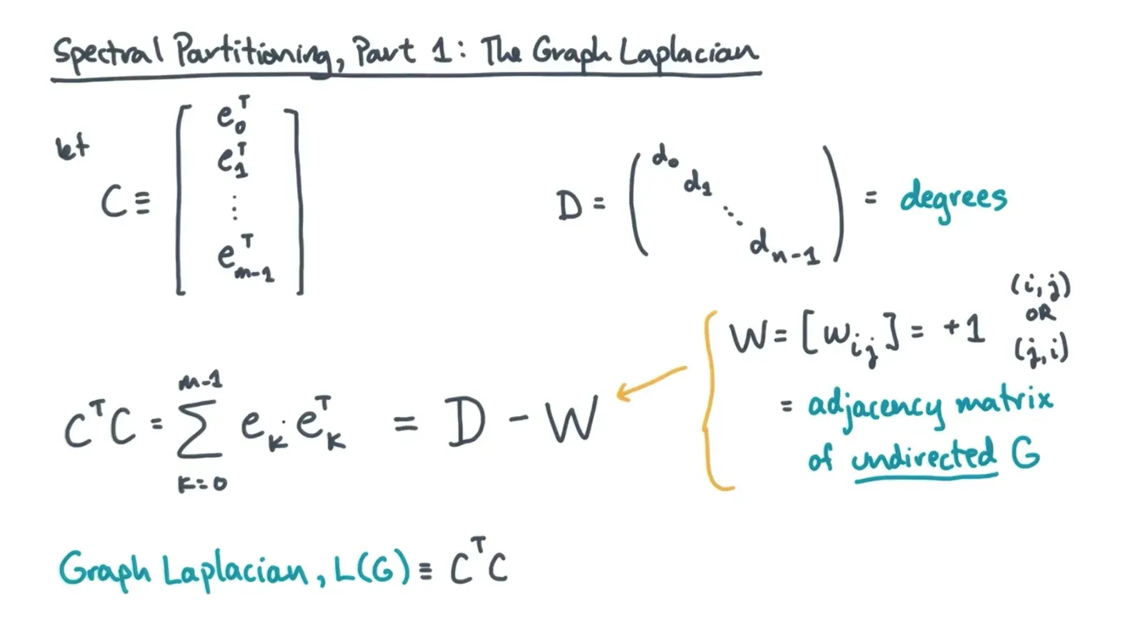
- The graph laplacian is its incidence matrix transposed * incidence matrix
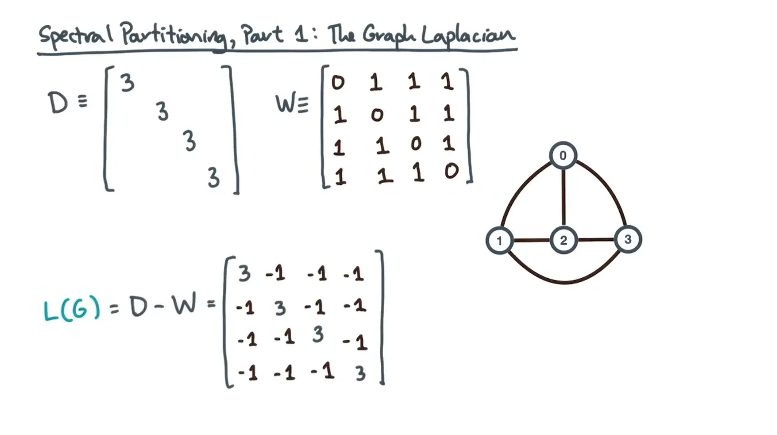
- The diagonals in the laplacian tell you incident edges on every vertex
- The sum or D(ignore direction treat as undirected) - W gives you the adjacency matrix of the undirected form of the graph
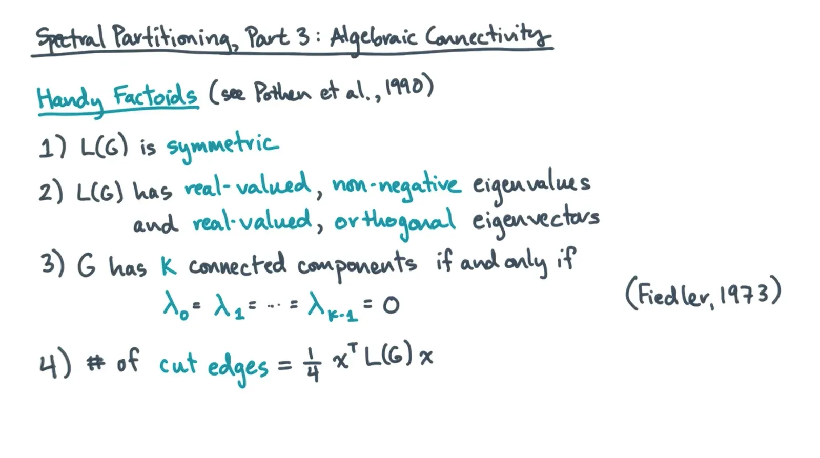
- Few facts related to the spectreal partitioning algorithm
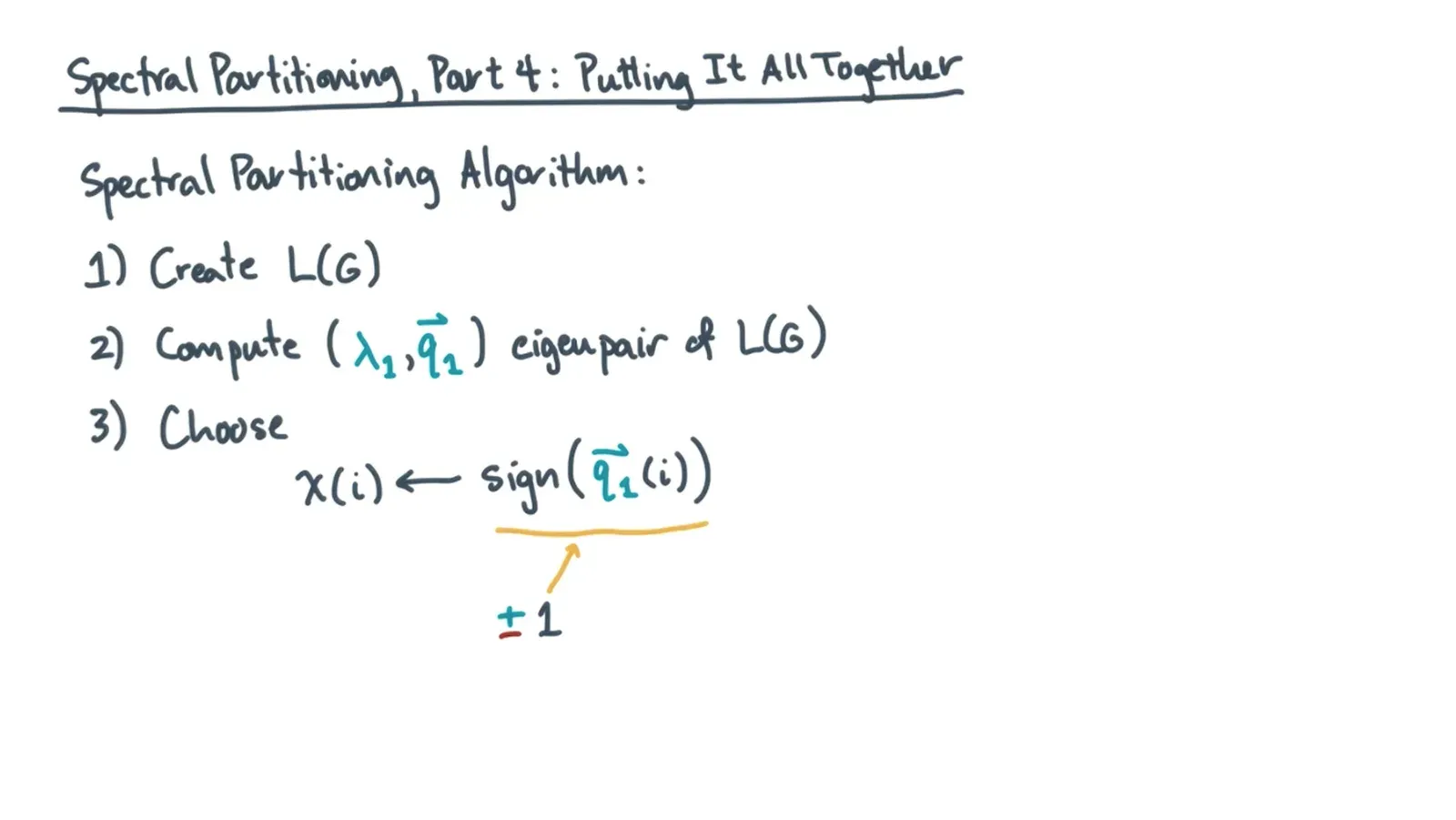
- Spectral partitioning algorithm
OPTIONAL: Algorithmic Time - Energy and Power
- Trend is that peak throughput doubles every 2 years
- To hit the speed of light in terms of cpu mesh operation travel distance then cpu has to be very very tiny
- The more data you want to store in memory, the smaller the size you must store a bit/byte is → at some point can’t squeeze in more data per bit so need to think about memory locality
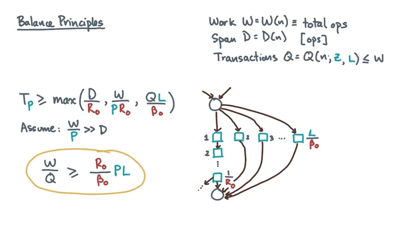
- The algorithms people should maximize W/Q or work over memory data transactions and hardware peopple should minimize machine balance or R/B or Transistors over Streams
- Power is the energy consumed / over a certain time period
- Total power is constant power (baseline power system uses when not doing anything) + dynamic power (power that system uses when performing operations)
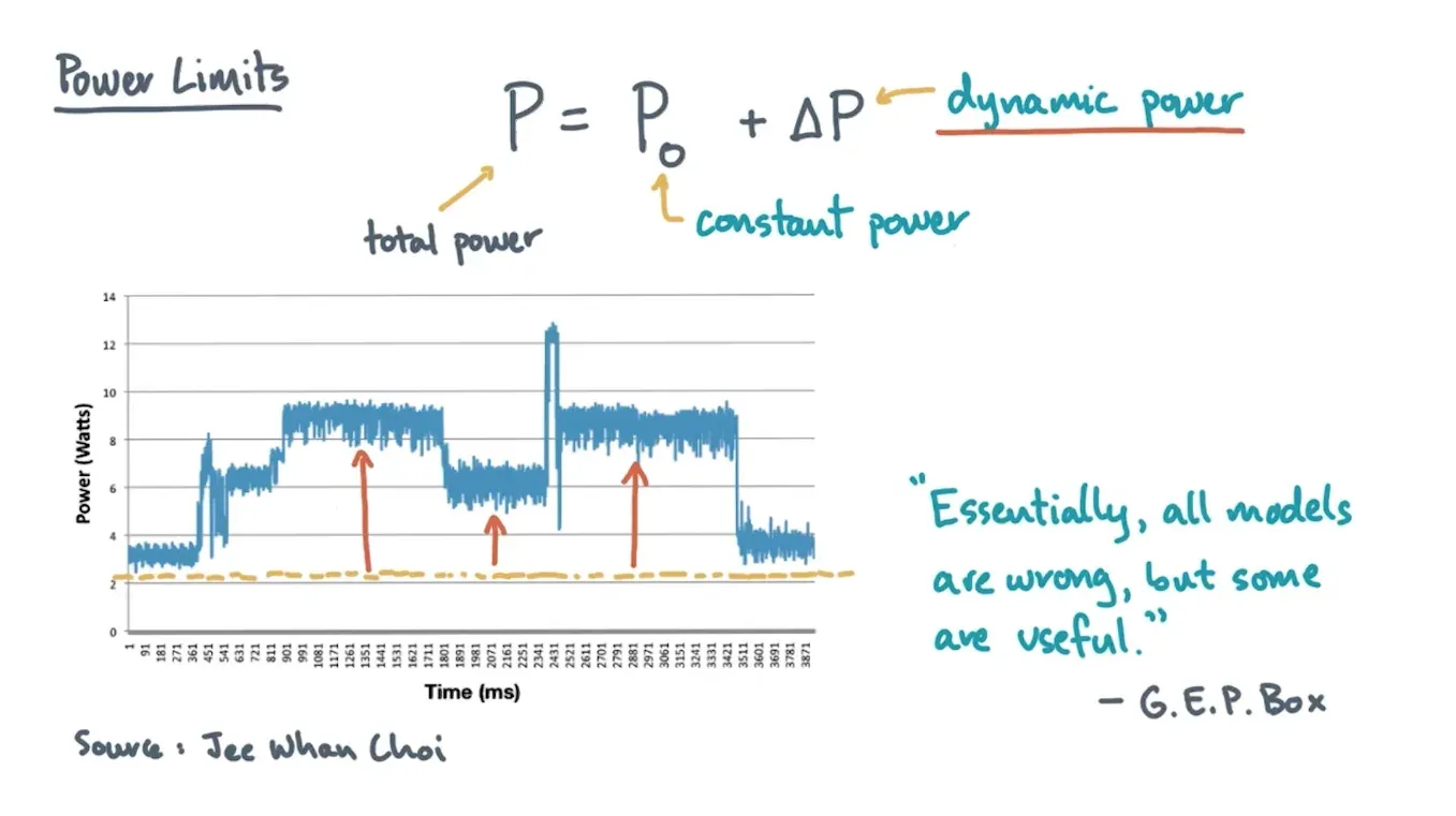
- Total power is constant power (baseline power system uses when not doing anything) + dynamic power (power that system uses when performing operations)
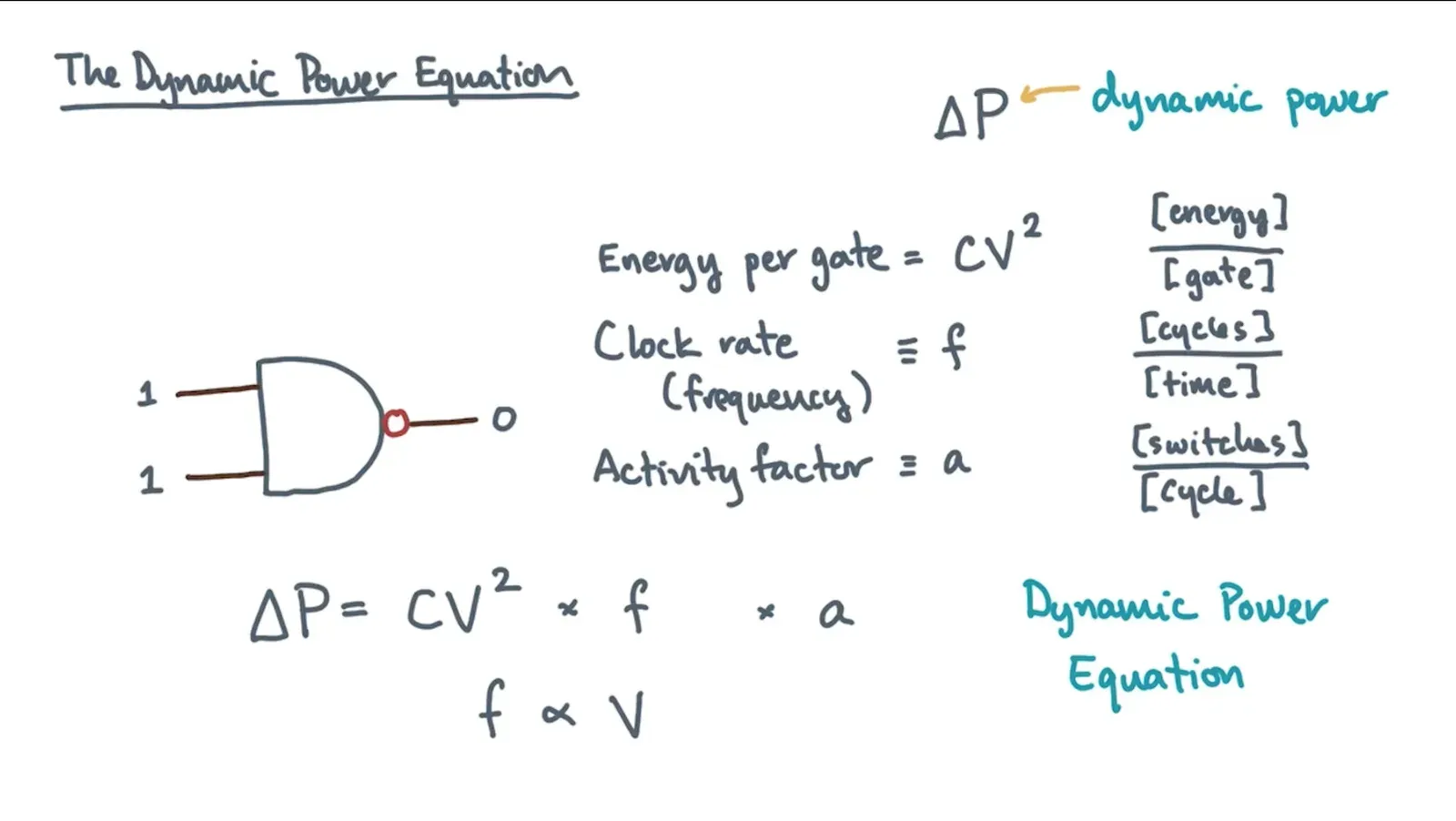
- Dynamic Power Equation = Energy per gate switch * clock rate frequency * activity factor
- Capacitance * Voltage ^ 2 * Frequency * Activity Factor
- Can take a lower frequency chip which runs at exponentially less power and paralellize this to emulate performance of a higher frequency chip running on significantly more power
OPTIONAL: Cache Obliviousness
- Normally in programming we write programs that let the cache automatically be managed by hardware and don’t care how the underlying cache does its thing ⇒ Cache Oblivious
- How can we model automatic fast memory and can an oblivious algorithm match IO performance on an aware algorithm?
- The ideal cache model makes a few assumptions
- When you do load/store operations, you access fast memory and if it’s not there then you load an entire cache line in memory → there are Z/L cache lines available
- Cache misses load L words or 1 line
- Associative cache allows any cache block to align at any block/line w/o restriction
- If the cache is full must design an eviction policy to evict cache line accessed further in the future
- On normal workloads LRU gets asymptotically close to optimal cache policy
- When you do load/store operations, you access fast memory and if it’s not there then you load an entire cache line in memory → there are Z/L cache lines available
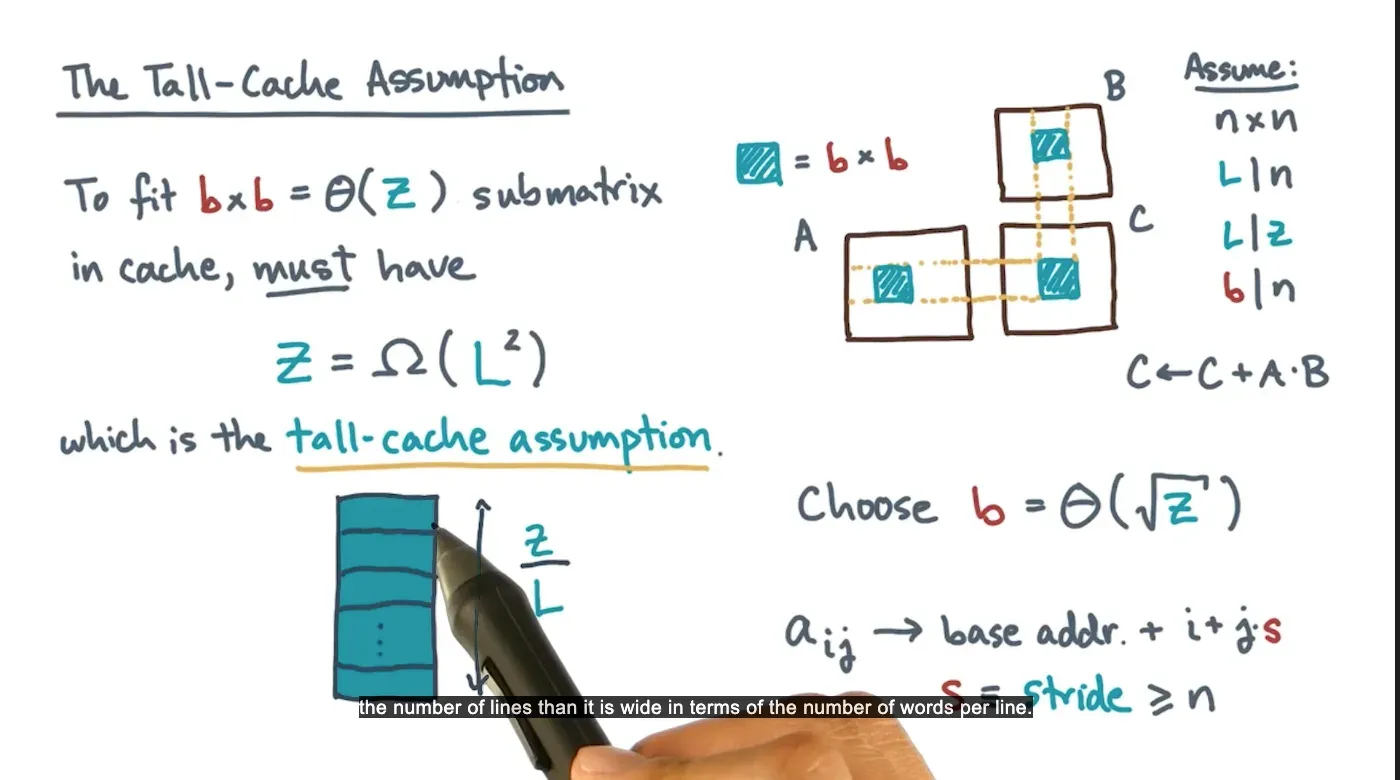
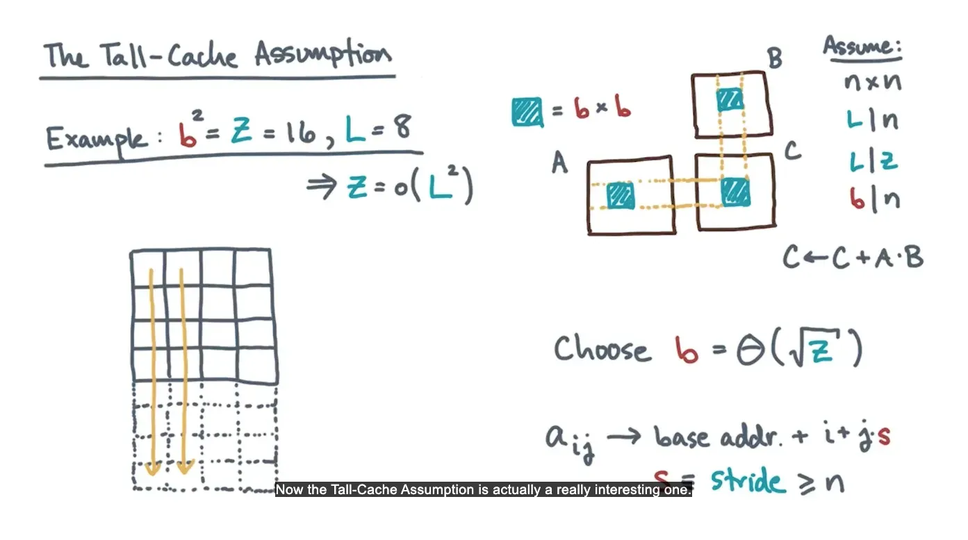
- Tall cache assumption assumes cache is taller in number of lines than it is wide in number of words per line
- If L^2 > Z then lines will not fit in cache
- If L^2 > Z then lines will not fit in cache
- Can perform cache oblivious (Straussen) matrix multiply and (Van Emde Boas) binary search
OPTIONAL: Shared Memory Parallel BFS
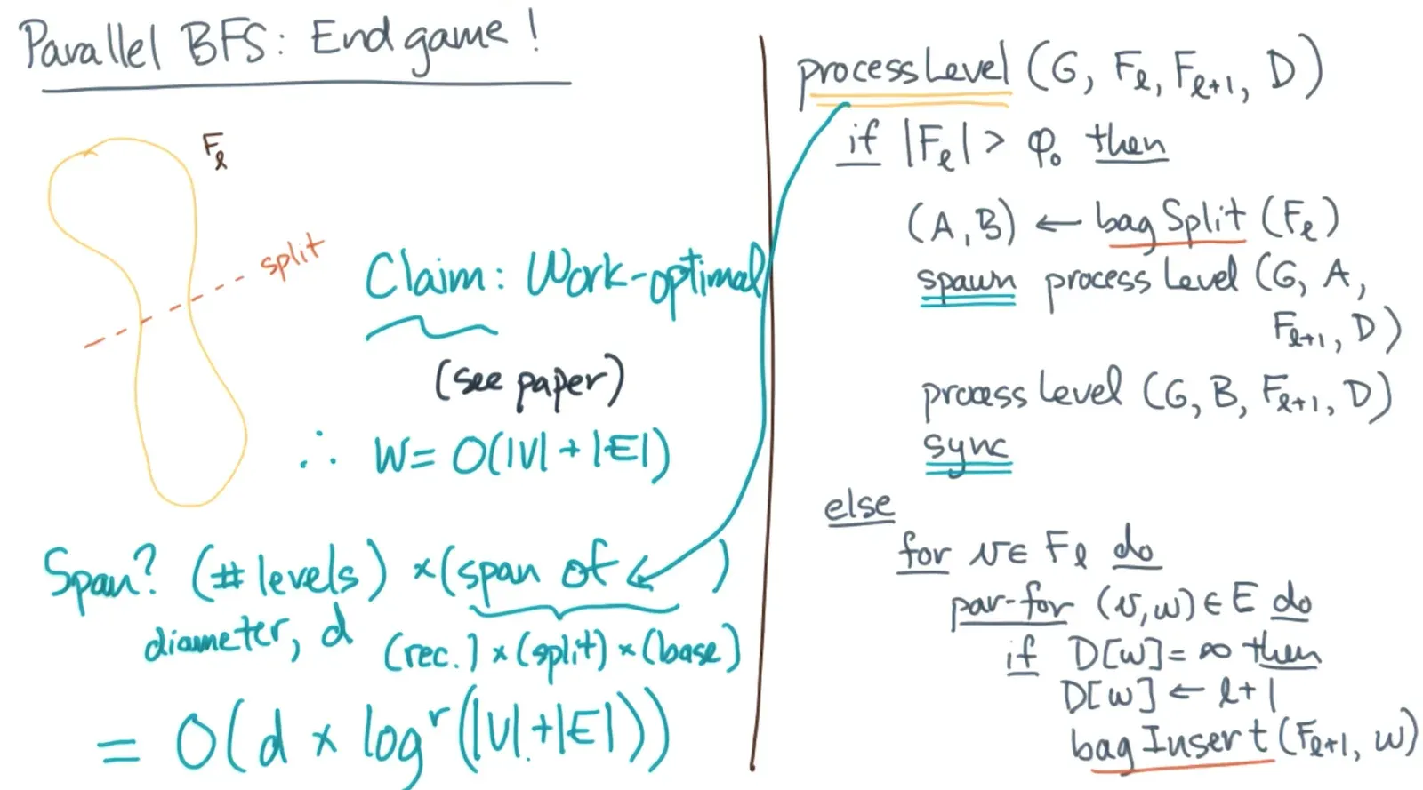
- The goal is to do a level order BFS traversal and process every level in parallel
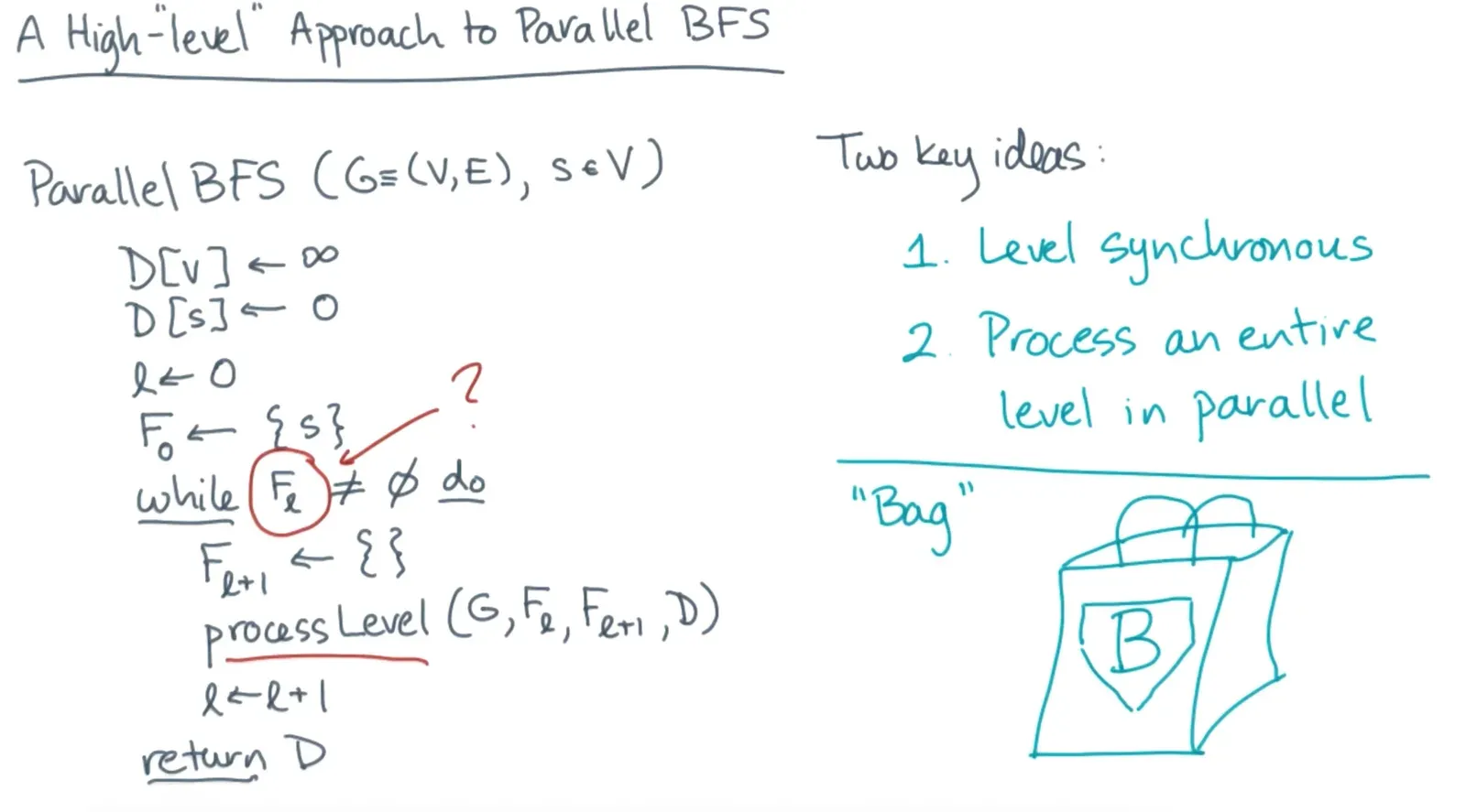
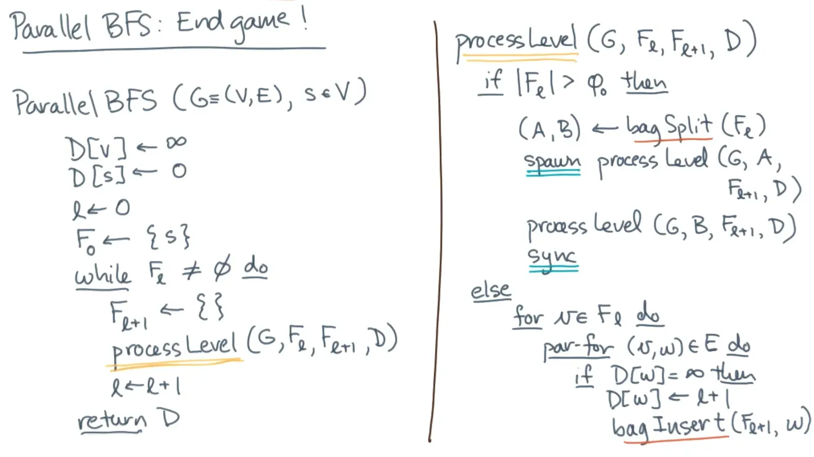
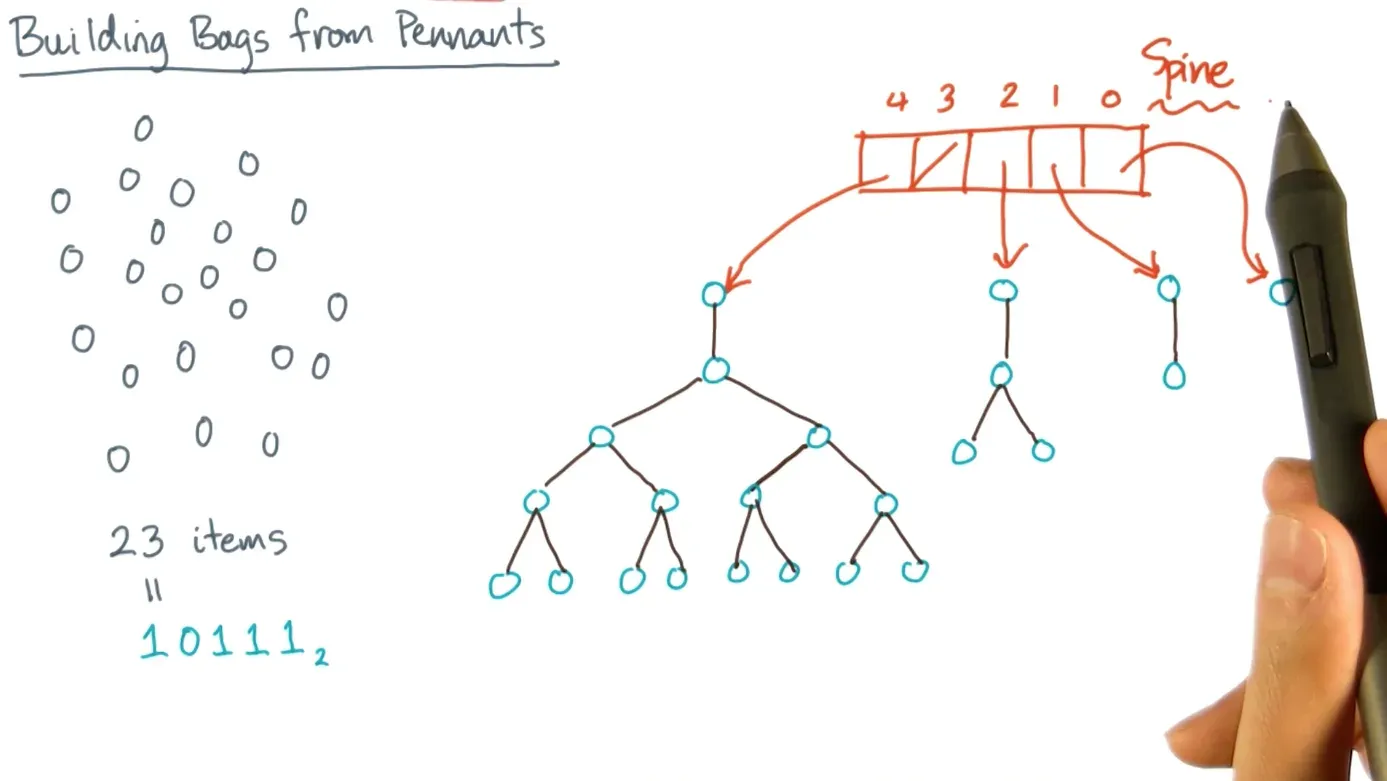
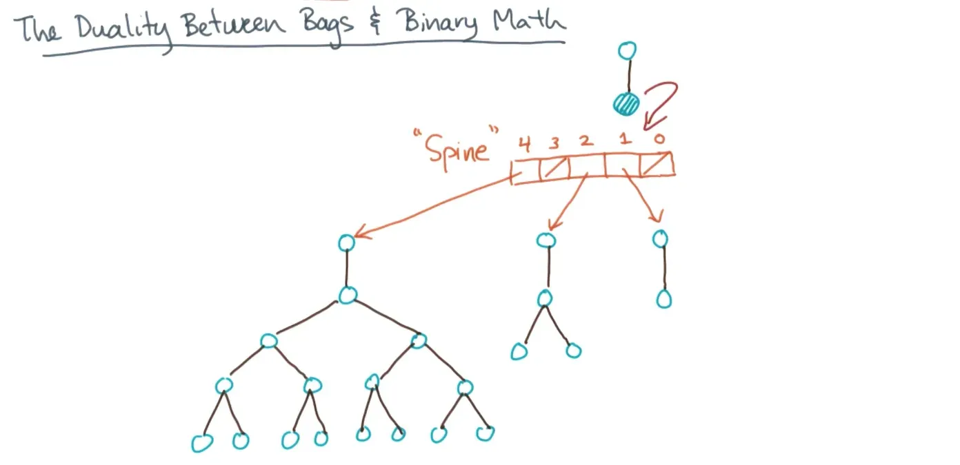
- Bags allow unordered collections with repetition - allowed since all duplicate vertices are at the same level
- Allows fast traversal and associative union and split operations
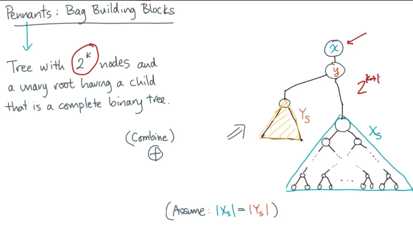
- 2 Pennants with 2^k nodes each and a complete binary tree can be combined in O(1) time by rearranging heads
Papers
- The Input/Output Complexity of Sorting and Related Problems
- Twelve Ways to Fool the Masses
- Lars Arge’s short summary of the sorting lower bound (2006)
- Chapter 27 (Multithreaded Algorithms) of Introduction to Algorithms
- Prefix Sums and Their Applications
- Designing Practical Efficient Algorithms for Symmetric Multiprocessors (Extended Abstract) — David R. Helman and Joseph JáJá
- Parallel Tree Contraction and its Applications
- Professor Tvrdik, Parallel Tree Contraction
- A Work-Efficient Parallel Breadth-First Search Algorithm (or How to Cope with the Nondeterminism of Reducers)
- Parallel Breadth-First Search on Distributed Memory Systems
- A Separator Theorem for Planar Graphs
- An Efficient Heuristic Procedure for Partitioning Graphs
- Parallel Multilevel k-Way Partitioning Scheme for Irregular Graphs
- Algebraic Connectivity of Graphs
- Partitioning Sparse Matrices with Eigenvectors of Graphs
- An Experimental Comparison of Pregel-like Graph Processing Systems